Including Births and Deaths

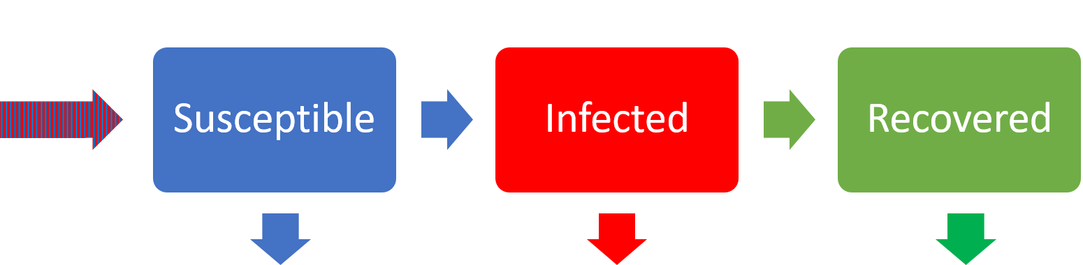
In our initial epidemic model in the previous chapter we had only two mechanisms involved – infection and recovery. Let us now add some increased detail into the model by including birth and death processes. Given the timescales of epidemic processes, this likely means looking at dynamics over a much longer time period, at least in human populations. Let’s begin by drawing a schematic of the system again:

We will make the simplifying assumption that the birth rate and death rate are equal, so that the population would be at equilibrium in the absence of disease (this is a questionable assumption for many ecological populations, but perhaps not too unreasonable for modern human populations). If we assume all individuals produce offspring at rate [latex]\mu[/latex], that everyone is born susceptible, and that every individual has the same death rate, also [latex]\mu[/latex], this leads us to the equations,

[latex]\begin{align} &\frac{dS}{dt} = \mu N - \beta SI - \mu S\\ &\frac{dI}{dt} = \beta SI - (\gamma +\mu)I\\ &\frac{dR}{dt} = \gamma I-\mu R \end{align}[/latex]

Once more, [latex]dN/dt=0[/latex] so we can eliminate [latex]R=N-(S+I)[/latex] (again, this is somewhat by design – if the rates of birth and death were not equal this simplification could not be made). One thing to note here is that the infectious period has changed to be [latex]1/(\gamma+\mu)[/latex]. When we define [latex]R_0[/latex], therefore, in our updated model we will have [latex]R_0=\beta N/(\gamma+\mu)[/latex].

Endemic disease

At this point we could non-dimensionalise our system as we have seen previously. This would allow us to reduce the number of parameters in our model to make life easier, as well as revealing potentially useful information about the scales involved. You will see some studies do this and others don’t. For now, let us continue with our analysis without doing so, since it means we retain the clear biological meanings of all of our parameters and variables.

First we should find the equilibria of our system, where [latex]dS/dt=0[/latex] and [latex]dI/dt=0[/latex] simultaneously. Recall in the previous model this only happened when [latex]I=0[/latex], with this condition satisfying both ODEs and leaving us with a line of equilibria. Now, we find more ‘standard’ unique equilibria. There are two cases where [latex]dI/dt=0[/latex]:

• [latex]I^*=0[/latex], giving [latex]dS/dt=0\implies S^*=N[/latex];

This means the population is disease-free.

•  [latex]S^*=\dfrac{\gamma+\mu}{\beta}[/latex], giving [latex]dS/dt=0\implies I^*=\dfrac{\mu(N-S^*)}{\beta S^*}=\dfrac{\mu}{\beta}\left(\dfrac{N}{S^*}-1\right)[/latex];

This means the disease is endemic.

We can do a bit more manipulation of that last equilibrium,

[latex]\begin{equation} I^*=\frac{\mu}{\beta}\left(\dfrac{N}{S^*}-1\right)=\frac{\mu}{\beta}\left(\frac{\beta N}{\gamma+\mu}-1\right)=\frac{\mu}{\beta}\left(R_0-1\right). \end{equation}[/latex]

While both expressions are equally correct, the latter one is nice in that [latex]R_0[/latex] is included in the expression. We now have two important terms from epidemiology. An epidemic occurs when a disease initially spreads through a population. A disease is endemic when it remains at a steady level within the population.

Having found these equilibria we now want to classify their stability. Let’s look at the Jacobian for our system,

[latex]\begin{align} J=&\left( \begin{array}{cc} -\beta I^*-\mu & -\beta S^*\\ \beta I^* & \beta S^*-(\gamma+\mu) \end{array} \right) \end{align}[/latex]

We shall now deal with each of our equilibria in turn.

Disease-free equilibrium

[latex]\begin{equation*} J=\left( \begin{array}{cc} -\mu & -\beta N\\ 0 & \beta N-(\gamma+\mu) \end{array} \right) \end{equation*}[/latex]

Having a zero in an off-diagonal (for a 2×2 matrix) makes our life much easier, as we can just read off the eigenvalues as the two diagonal entries. In this case we therefore have [latex]\lambda_1=-\mu[/latex] and [latex]\lambda_2=\beta N-(\gamma+\mu)=(\gamma+\mu)(R_0-1)[/latex]. Therefore, if [latex]R_0\lt1[/latex], the disease-free equilibrium is unstable.

Endemic equilibrium

[latex]\begin{equation*} J=\left( \begin{array}{cc} - \mu R_0& -(\gamma+\mu)\\ \mu(R_0-1)& 0 \end{array} \right) \end{equation*}[/latex]

In this case we cannot read off our eigenvalues, so we shall instead look at the signs of the trace and determinant:

• [latex]tr(J) = -\mu R_0\lt 0[/latex]
• [latex]\det(J) =\mu(\gamma+\mu)(R_0-1)[/latex]

Since the trace is always negative, from the determinant we see that if [latex]R_0\gt 1[/latex], the endemic equilibrium is stable.

The stable equilibrium can be a node or a spiral depending on the precise parameter values. Generally, high [latex]\gamma[/latex], intermediate [latex]R_0[/latex] and low [latex]\mu[/latex] make a spiral more likely.

Putting these results together we can see that when [latex]R_0\gt 1[/latex] the disease will become endemic.

Phase portraits

We can explore these two scenarios further with phase portraits. First we remember that again we must have [latex]S+I\le N[/latex], so we only have a triangular region in our phase portraits to really worry about. To find the nullclines:

[latex]\begin{align*} &dS/dt=0\implies I=\frac{\mu}{\beta}\left(\frac{N}{S}-1\right)\\ &dI/dt=0\implies I=0,S=\frac{\gamma+\mu}{\beta}. \end{align*}[/latex]

Click for solution

The two phase portraits are sketched below. If you start sketching a phase portrait you should find that the only way you can produce two qualitatively different phase portraits is again about the placement of the vertical nullcline, now given by [latex]S=(\gamma+\mu)/\beta[/latex], which in turn relates to whether or not [latex]R_0\gt1[/latex] or not. In the first diagram, all trajectories will eventually approach the bottom-right corner at the disease-free equilibrium. In the second diagram, you should see the new endemic equilibrium in the middle where the two nullclines cross. Trajectories approach this equilibrium, moving around it anti-clockwise (as I once read, if you can’t remember clockwise/anti-clockwise directions, clockwise is the way you dial a phone).

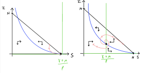
We see nice demonstrations of the behaviour we predicted from our stability analysis here. In particular, when [latex]R_0\gt 1[/latex] the disease will persist in the long-term.

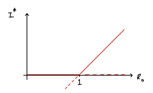
[latex]R_0[/latex] is a quantity that is often estimated for diseases when they emerge, and gives a good indication of how contagious they are and (as we shall see below) how easy they will be to eradicate. We can also use [latex]R_0[/latex] as a useful bifurcation parameter to draw a bifurcation diagram of this system below. Note again the key value of [latex]R_0=1[/latex] where the transcritical bifurcation occurs.

Vaccination

Suppose we want to prevent a disease spreading through a vaccination programme. What proportion, [latex]p[/latex], of the population do we need to vaccinate to succeed? If our vaccine works perfectly then the pre-infection density of susceptibles reduces from [latex]N[/latex] to [latex]N(1-p)[/latex]. Recall that for the disease to die out we want [latex]R_0=\beta N/(\gamma+\mu)\lt 1[/latex]. After vaccination this becomes,

[latex]\begin{align*} \frac{\beta N(1-p)}{\gamma+\mu} \implies p\gt 1-\frac{1}{R_0} \end{align*}[/latex]

Note that not all of the population needs to be vaccinated – just enough to prevent the disease from spreading freely. This is important as there may be certain groups, those undergoing medical treatment, for example, who cannot be vaccinated. This population-wide protection created by significant vaccination is called herd immunity. The higher the [latex]R_0[/latex] of the disease, the greater proportion of the population that needs to be vaccinated.

A point about herd immunity

This method to calculate the herd immunity threshold relies on using [latex]R_0[/latex] as our key parameter, which is the relative speed of spread if the initial population is disease-free. During the Covid-19 pandemic, proposals were made for a “herd immunity strategy” that would essentially rely on the disease dying away once enough of the population – the herd immunity threshold – had immunity, but immunity that was acquired after being infected, not through vaccination. There are two big drawbacks to this approach (see chapter references).

Firstly, as we have seen here, if the disease persists for any length of time – such that birth and death processes start to introduce population turnover – we’d be unwise to assume the disease would naturally burn out. There are a whole host of other factors that would also allow for a disease to persist in the long-term, including waning immunity and lack of immunity to mutations to name just two.

Secondly, and related to [latex]R_0[/latex], if we use the herd immunity threshold as calculated above, the idea is that we have protected (almost) the whole population until a vaccine was developed, and then we can move enough individuals out of the susceptible compartment to stop the disease from ever spreading. If instead we allow the disease to spread the key parameter is no longer [latex]R_0[/latex] but [latex]R_t[/latex], as discussed in the last chapter. We know [latex]R_t[/latex] equals 1 exactly at the peak of an epidemic, and at this point the proportion that has been infected will be the same as the herd immunity threshold. However, in this approach we now have a potentially large proportion of the population who are still infected, as well as a large proportion who remain susceptible. So while the number of infections will start to fall (because we are in the region of [latex]R_t\lt1[/latex]) we will still have a considerable number of onward infections. Say that we calculate that a disease has [latex]R_0=3[/latex], meaning the herd immunity threshold is 66.7%. As we have just said, that is now the proportion that has been infected at the peak of the infection. By the time the infection has actually died out, the proportion infected will be over 90%.

The lesson here is to be careful about how you interpret models!

Chapter references

• The discussion on herd immunity is based on the paper by Best & Ashby (2022).
• The content in the Infectious diseases section was influenced by the textbooks, Mathematical Biology 1 by Murray and Modelling Infectious Diseases in Humans and Animals by Keeling & Rohani.