A first population model

Our aim in this textbook is to model the dynamics of populations over time. By ‘population’ we simply mean some collection of individuals that are subject to the same underlying mechanisms. For example, we may consider the human population of Sheffield, or the tapir population of South America, or the maize crop population of a field in Nigeria. In later chapters we will move to smaller biological scales, considering perhaps less intuitive definitions of populations, such as of cells in the body, or proteins within cells. However, a key message to take from this textbook is that we can consider pretty much any biological populations in the same way from a modelling perspective, and subject to the same fundamental biological mechanisms.

We will model these dynamics using ordinary differential equations, and our focus will be on how the size of a population varies over time. We will not consider where individuals are in space – this would likely require extending our methods to partial differential equation models, and plenty of excellent courses and textbooks can be found to explore such systems. When we talk about the ‘size’ of a population, we might think we mean the number of individuals. However, as we will be using ordinary differential equations we need our variables to be continuous, not discrete. We will therefore instead keep track of a population’s density – the number of individuals within some unit area.

Introducing our mathematical notation, we might call [latex]N(t)[/latex] the density of individuals within our population at time [latex]t[/latex]. We now wish to write down an ordinary differential equation that describes its dynamics – that is what causes the population to increase or decrease. Our first modelling challenge, then, is to decide what mechanisms we should include. What mechanisms would lead a population to change in size? Using some biological intuition for the simplest possible population we can think of, we might expect our model to look something like,

[latex]\begin{align} \frac{dN}{dt} &= \textrm{births} -\textrm{deaths}. \end{align}[/latex]

Now to make any mathematical progress we will need to decide on functional forms for each of these mechanisms. This is another important modelling decision, and will depend on the specific biology. There are three main forms we might use:

• constant rate, [latex]\textrm{births}=b[/latex]. This would be suitable when new individuals appear in the environment at some constant rate, for example due to migration, or production of cells by the body.
• per-capita rate, [latex]\textrm{births}=bN[/latex]. This would be suitable when each individual produces offspring at a certain rate, such that there are more offspring produced when the population is larger.
• density-dependent rate, [latex]\textrm{births}=b(N)N[/latex]. This would be suitable if the per-capita rate is not fixed but instead varies with the population size, for example if high density means more competition for resources and thus lower growth. The form of this function will again depend on the biology, though there are common functions we tend to use.

For our basic model, per-capita rates for birth and death seem the most obvious choice. Our model is thus,

[latex]\begin{align} \frac{dN}{dt}&= bN - dN \\ &= rN, \end{align}[/latex]

where the parameter [latex]r=b-d[/latex] is the growth rate of our population. We therefore have a first-order, linear ordinary differential equation (ODE). Such ODEs are readily solved using either separation of variables or integrating factors. In this textbook I have made the assumption that readers are comfortable with such methods. If you are not, you might like to look at a textbook or online material for solving linear ordinary differential equations, but in the first few exercises I will also provide fairly detailed worked solutions. Have a go at the exercise below to solve this first population model.

This predicts exponential growth of the population for [latex]r\gt0[/latex] and exponential decline for [latex]r\lt0[/latex].

The logistic equation

We would usually assume that births are greater than deaths, meaning [latex]r\gt0[/latex] and our population will continue growing to infinitely large densities. This is, we can hopefully agree, a tad unrealistic. We should not lose heart at this point, though. A model that produces unrealistic results is still helpful to us, because it will point the way towards how we can develop an improved version (remember the adage, all models are wrong but some are useful).

What might we have failed to take into account in our model? One answer is that as the population grows the environment will become limiting in some way. For example, individuals need space and nutrients to live. These resources will be consumed by the population more and more as the population grows, likely leading to reduced birth or increased death rates. So while our assumptions may hold at low population densities, they will break down at higher densities. Our simple model has shown us that we need to take this into consideration if we are to understand the population dynamics.

Given this, choosing a density-dependent growth rate starts to look like a better assumption. A relatively simple and intuitive way to set a limit on population growth is to assume that there is a fixed carrying capacity for the population, for example due to the available space or nutrients. We assume that as the population approaches this carrying capacity, the overall growth rate approaches zero, and once the population goes above this value the growth rate becomes negative. The simplest implementation of this is to assume that [latex]r[/latex] decreases linearly with [latex]N[/latex]:

[latex]\begin{equation} r(N) = r_0\left(1 - \frac{N}{K}\right), \end{equation}[/latex]

where [latex]r_0[/latex] (the basic reproductive rate) and [latex]K[/latex] (the carrying capacity) are positive constants. Our ordinary differential equation for the dynamics of our population is then

[latex]\begin{equation} \frac{dN}{dt}=r_0N\left(1 - \frac{N}{K}\right). \end{equation}[/latex]

This equation is known as the logistic growth equation and is an example of intra-specific competition.

A useful step: non-dimensionalisation

We can continue our analysis with the model in this form again using methods for solving ordinary differential equations. However, before continuing with our analysis we shall introduce the useful technique of non-dimensionalising our model. This is often – though by no means always – done to models to simplify some of the later working. It can both reduce the number of parameters in the model and give us insight in to the scales at which biological processes operate.

Non-dimensionalisation involves combining variables and/or parameters from the model in biologically and mathematically helpful ways. For example, a natural scale for the population level is [latex]K[/latex], so we can define the non-dimensional population variable [latex]n=N/K[/latex] ([latex]n[/latex] is non-dimensional because both [latex]N[/latex] and [latex]K[/latex] have units 1/[density], so [latex]n[/latex] is a dimensionless number). The equation then becomes

[latex]\begin{equation} \frac{dn}{dt}=\frac{d(N/K)}{dt}=\frac{1}{K}\frac{dN}{dt}=r_0n(1 - n). \end{equation}[/latex]

We can also note that a natural time scale for the dynamics is [latex]1/r_0[/latex], such that we can take a new non-dimensional time variable, [latex]\tau = r_0t[/latex], and the final non-dimensional model equation is

[latex]\begin{equation} \frac{dn}{d\tau}=\frac{dn}{d(r_0t)}=\frac{1}{r_0}\frac{dn}{dt}=n(1 - n). \end{equation}[/latex]

As you can see, by using two substitutions we have arrived at a very simple equation.

Model analysis

Even though this equation is non-linear (we have an [latex]n^2[/latex] term), we can still find an explicit solution for it. By separation of variables, we can write this as,

[latex]\begin{equation} \int\frac{dn}{n(1-n)} = \int r_0 d\tau, \end{equation}[/latex]

We cannot immediately integrate the left-hand side of this. However, we can use partial fractions to rewrite the fraction on the left-hand side as the sum of two terms (it turns out to be [latex]1/n+1/(1-n)[/latex]). We can now integrate these to reach an initial solution of,

[latex]\begin{align} &\ln(n)-\ln(1-n) = r_0\tau+C,\\ \implies &\frac{n}{1-n}=e^Ce^{r_0\tau}, \end{align}[/latex]

where [latex]C[/latex] is a constant of integration. Letting the initial condition be [latex]n(0)=n_0[/latex] and rearranging, we arrive at the final solution,

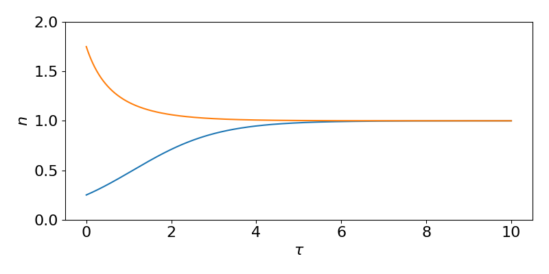
[latex]\begin{equation} n(\tau) = \frac{n_0}{n_0+(1-n_0)e^{-\tau}}. \end{equation}[/latex]

(Alternatively a suitable substitution can be chosen to evaluate the integrals. It is often true in mathematical modelling that there are multiple ways to arrive at a solution, and embracing this diversity of approach can be very useful).

Examples of the (non-dimensional) solution for two different initial densities are shown in the figure.

While this has been useful to get an explicit solution, we can in fact gain a good deal of qualitative information about this model directly from the ODE without having to spend the few minutes involved in deriving that explicit solution. Specifically, we can see:

• for [latex]0\lt n\lt 1[/latex], [latex]dn/d\tau \gt 0[/latex],
• for [latex]n \gt 1[/latex], [latex]dn/d\tau \lt 0[/latex],

(note that it makes no biological sense to worry about [latex]n\lt0[/latex]). There are two values of [latex]n[/latex] for which [latex]dn/d\tau=0[/latex], at [latex]n=0[/latex] and [latex]n=1[/latex], which are the equilibria of the system. Therefore for any starting value of [latex]n>0[/latex] the population should move towards a final state of [latex]n=1[/latex], suggesting that the equilibrium at [latex]n=0[/latex] is unstable and the equilibrium at [latex]n=1[/latex] is stable. We can think about this more by sketching the curve [latex]dn/d\tau[/latex] vs [latex]n[/latex]. If you are unfamiliar with linear stability analysis you should have a read of the relevant background review chapter.

Click for solution

On this sketch we can mark our equilibria at [latex]n=0[/latex] and [latex]n=1[/latex] and then consider the wider behaviour by considering the curve [latex]dn/d\tau[/latex] as a function of [latex]n[/latex]. The highest power here is [latex]n^2[/latex] so the curve will look like a quadratic, and since the [latex]n^2[/latex] term is negative it will initially increase, then peak, and then decrease.

For convenience let us call [latex]dn/d\tau=f(n)[/latex], and then look at what happens nearby the equilibria by linearisation.

• At [latex]n=0[/latex], the gradient of the curve [latex]df/dn[/latex] is positive, meaning [latex]dn/d\tau\gt 0[/latex] for [latex]n \gt 0[/latex] and [latex]dn/d\tau\lt 0[/latex] for [latex]n \lt0[/latex] (we don’t really mind about the actual values in this latter case since [latex]n \lt 0[/latex] but it helps for picturing the gradient). As such if we start with a population density a small distance away from [latex]n=0[/latex] we will always end up moving further away from it – it is unstable.
• At [latex]n=1[/latex], we have [latex]df/dn[/latex] negative, meaning [latex]dn/d\tau\gt 0[/latex] for [latex]n\lt 1[/latex] and [latex]dn/d\tau\lt 0[/latex] for [latex]n\gt 1[/latex], As such if we start with a population density a small distance away from [latex]n=1[/latex] we will always move in towards this equilibrium – it is stable.

We can also mark on the qualitative direction of trajectories on the x-axis, giving a phase line. Notice, then, that we have fully described the possible behaviours of this system without having to explicitly solve the equation.

Case study: spruce budworm

Spruce budworm is an insect that lives in spruce and fir forests in the USA and Canada (see chapter references). While they mostly exist at low numbers, there are periodic explosions of budworm populations that devastate the forests. Let us assume that on their own, the budworm populations follow the logistic growth model we have just studied. An additional feature of budworm dynamics is that they are predated by birds. We might then describe the dynamics of budworm by the following equation,

[latex]\begin{equation} \frac{dN}{dt}=r_0N\left(1 - \frac{N}{K}\right)-P(N), \end{equation}[/latex]

where [latex]P(N)[/latex] describes the rate of predation (note that we do not explicitly consider the bird population dynamics). What should [latex]P(N)[/latex] look like? Should it be constant, a fixed per-capita rate, or some other density-dependent function? First, we might reasonably assume that as more food becomes available, the more the birds will eat, so predation should increase with budworm density. However, birds cannot eat an infinite amount, and so the rate of predation should therefore saturate at high budworm densities. We therefore need a density-dependent function. We might then give an explicit model as,

[latex]\begin{equation} \frac{dN}{dt}=r_0N\left(1 - \frac{N}{K}\right)-\frac{\rho N}{N+A} \end{equation}[/latex]

This form for the predation function is a very commonly used one in mathematical biology models  (in this context it is often known as a Holling type II functional response). What are the possible outcomes of this model? We might start by finding equilibria as before, but we will quickly find ourselves bogged down. Instead, let’s take a qualitative approach and use curve-sketching to explore the possible outcomes. The above model can be written as,

[latex]\begin{equation} \frac{dN}{dt}=N\left[r(N)-p(N)\right], \end{equation}[/latex]

where [latex]r(N)=r_0(1-N/K)[/latex] and [latex]p(N)=\rho/(N+A)[/latex]. We know that an equilibrium occurs where [latex]r(N)-p(N)=0[/latex], which will be when the two curves cross. Below we sketch these two curves, [latex]r(N)[/latex] and [latex]p(N)[/latex], for the three possible orientations, separated by how high the predation parameter [latex]\rho[/latex] is.

It is worth stressing that [latex]N=0[/latex] is always an equilibrium even though the two curves may not cross here – if you look back at the ODE we factored [latex]N[/latex] out of the equation. What happens in each case?

1. Predation by the birds is very high, the two curves never cross, and [latex]dN/dt \lt 0[/latex] for all [latex]N>0[/latex]. Therefore the insect population is always reducing until it reaches extinction, with [latex]N=0[/latex] a stable equilibrium.
2. Predation has weakened somewhat and two new equilibria appear, one stable and one unstable. We now have bistability – where two different equilibria are stable, but which one we go to depends on the initial conditions.
3. Predation is very weak and we now only have one equilibrium for [latex]N\gt 0[/latex], at high budworm densities. We also see now that [latex]N=0[/latex] is no longer stable, and the budworm population will always reach this high equilibrium density.

What do these results tell us? That pest outbreaks such as spruce budworm are likely to be driven by the pressure from predation. We can also see that, due to the bistability, sudden outbreaks can occur if there are relatively small changes to the environment. We have achieved this insight without having to do any detailed mathematical derivations, but by applying mathematical reasoning and biological interpretation – these are two key skills we will develop over this course.

Bifurcation diagram

This model reveals that as we alter a parameter value, the behaviour of the model qualitatively shifts, either through switching the stability of two already existing equilibria or through the creation of completely new equilibria. Such transitions are called bifurcations, which you can read further on in the relevant background chapter if needed. A useful approach is to draw a bifurcation diagram, which effectively puts all of the information on our diagrams above into one single plot, allowing us to see at a glance what the possible behaviours and transitions are. The bifurcation diagram for this model is shown below.

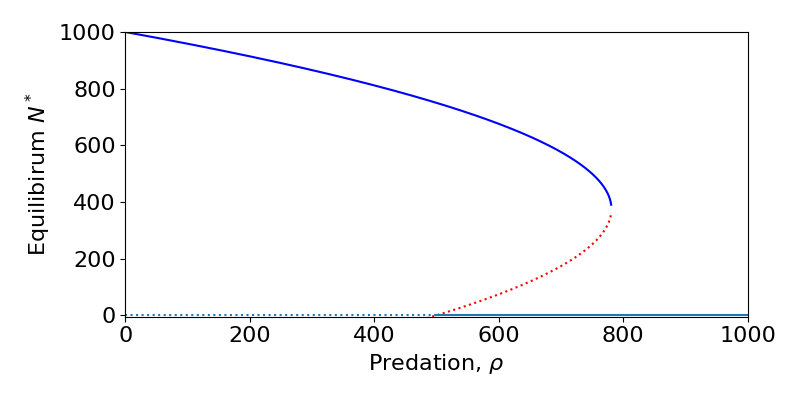
This shows that if [latex]\rho[/latex] is small, we have two equilibria – one at [latex]N^*=0[/latex] that is unstable and one for high [latex]N^*[/latex] that is stable. Therefore throughout this region, the population will be attracted to the equilibrium with a large population (though its value shrinks as predation increases). At [latex]\rho=100[/latex] a transcritical bifurcation occurs where a further equilibrium (that was at negative values and so hadn’t been drawn) collides with [latex]N^*=0[/latex] – causing itself to be unstable and the zero equilibrium to become stable – and then increases. In this second region we therefore have bistability between extinction and the higher (but again, decreasing) equilibrium. At around [latex]\rho=300[/latex] the two non-zero equilibria collide and disappear in a saddle-node bifurcation. This leaves the final region where only the extinction equilibrium exists and is stable.

Chapter references

• The spruce budworm model is based on an example from the textbook, Mathematical Biology 1 by Murray.
• The content in the Population ecology section was influenced by the textbook, Mathematical Biology 1 by Murray.