
20 A two compartment bolus model
A bloodstream-tissue model
For our final chapter (well done for making it!) we will return to the scenario of intravenous bolus doses. In our earlier models we assumed the body acted as a single compartment for the drug, basically considering the drug concentration in the bloodstream. When we looked at the orally administered drug models we assumed there was now a second compartment where the drug had to enter the body (the GI tract) before it could move on to the bloodstream. In that case things simplified because the dynamics of the first compartment were very simple – exponentially decreasing to zero – and only concentrate on what happened in the bloodstream.
Now we will consider a more complicated case where there are two compartments, but the drug can now move in and out of both of those compartments. A biological example might be the bloodstream as our main compartment, and tissue as the second compartment. We will assume the drug is again administered by an intravenous bolus and so appears immediately in the bloodstream. The concentration of the drug in the bloodstream will again be given by [latex]C[/latex], and the concentration in the tissues will be given by [latex]D[/latex]. While in the bloodstream the drug is used up and is eliminated. The drug can also pass in to tissues at some rate [latex]a[/latex] and can pass back from tissues to the bloodstream at rate [latex]b[/latex]. We will assume the drug is not eliminated while in the tissue. Our mathematical model will thus look like,
[latex]\begin{align} \frac{dC}{dt}&=-kC-aC+bD\\ \frac{dD}{dt}&=aC-bD. \end{align}[/latex]
Solving a system of linear equations
Since both equations explicitly depend on both variables, we cannot handle this case in quite the same way as the previous pharmacokinetic models. We also cannot solve the system one equation at a time – i.e. apply an integrating factor to solve one, then substitue that solution into the second. However, we have a well established toolbox for dealing with a system of linear ordinary differential equations. I have not provided any explicit background review material for these methods, but will try to take the explanations quite slowly.
First note that we can write this out in matrix form, that is,
[latex]\begin{equation*} \frac{d}{dt}\left(\begin{array}{c}C\\D\end{array}\right)=\left(\begin{array}{cc}-k-a &b\\a & -b\end{array}\right)\left(\begin{array}{c}C\\D\end{array}\right). \end{equation*}[/latex]
For a system like this we expect to see solutions of the form,
[latex]\begin{equation} \left(\begin{array}{c}C(t)\\D(t)\end{array}\right)=\left(\begin{array}{c}u_1\\u_2\end{array}\right)e^{\lambda_1 t}+\left(\begin{array}{c}v_1\\v_2\end{array}\right)e^{\lambda_2 t}. \end{equation}[/latex]
This has become an eigenvalue/eigenvector problem since, substituting these desired solutions into our matrix equation we have,
[latex]\begin{equation} \lambda_1\left(\begin{array}{c}u_1\\u_2\end{array}\right)e^{\lambda_1 t}=\left(\begin{array}{cc}-k-a &b\\a & -b\end{array}\right)\left(\begin{array}{c}u_1\\u_2\end{array}\right)e^{\lambda_1 t}, \end{equation}[/latex]
and similarly for [latex]\lambda_2[/latex].
To solve such a problem we first find the eigenvalues. Calling the matrix of parameters [latex]M[/latex], we set [latex]\det(M-\lambda I_2)=0[/latex], where [latex]I_2[/latex] is the two-dimensional identity matrix, which leads to the characteristic equation,
[latex]\begin{equation} \lambda^2+(k+a+b)\lambda+kb=0. \end{equation}[/latex]
This does not factorise particularly nicely. Let us simplify things a little by choosing some new constants [latex]\alpha[/latex] and [latex]\beta[/latex] such that,
[latex]\begin{align} \alpha+\beta&=k+a+b\\ \alpha\beta&=kb. \end{align}[/latex]
This helps as it means the characteristic equation is now,
[latex]\begin{equation} \lambda^2+(\alpha+\beta)\lambda+\alpha\beta=(\lambda+\alpha)(\lambda+\beta)=0, \end{equation}[/latex]
for which the solutions are just [latex]\lambda=-\alpha[/latex] and [latex]\lambda=-\beta[/latex]. If and when the time comes to find out what values [latex]\alpha[/latex] and [latex]\beta[/latex] take, we would need to substitute them in to the quadratic formula to find,
[latex]\begin{equation} \alpha,\beta=\frac{(\alpha+\beta)\pm\sqrt{(\alpha+\beta)^2-4\alpha\beta}}{2}, \end{equation}[/latex]
and we have defined both [latex]\alpha+\beta[/latex] and [latex]\alpha\beta[/latex] in terms of the parameters [latex]a[/latex], [latex]b[/latex] and [latex]k[/latex] that we do know.
We have therefore narrowed down our general solution to be,
[latex]\begin{equation} \left(\begin{array}{c}C(t)\\D(t)\end{array}\right)=\left(\begin{array}{c}u_1\\u_2\end{array}\right)e^{-\alpha t}+\left(\begin{array}{c}v_1\\v_2\end{array}\right)e^{-\beta t}. \end{equation}[/latex]
To find the eigenvectors we substitute each eigenvalue back in and solve,
[latex]\begin{equation} \left(\begin{array}{cc}-k-a-\lambda &b\\a & -b-\lambda\end{array}\right)\left(\begin{array}{c}u_1\\u_2\end{array}\right)=\left(\begin{array}{c}0\\0\end{array}\right). \end{equation}[/latex]
Let us take [latex]\lambda=-\alpha[/latex]. Using the bottom line this gives the equation,
[latex]\begin{equation} au_1+(\alpha-b)u_2=0\implies au_1=(b-\alpha)u_2. \end{equation}[/latex]
Thus for some constant, [latex]\kappa_u[/latex], taking [latex]u_1=\kappa_u(b-\alpha)[/latex] and [latex]u_2=\kappa_ua[/latex] will always satisfy this. (An aside: you might wonder why we used the bottom line here and not the top. When dealing with these eigenvector problems we usually expect to get basically the same expression whichever line we use, but here it is not obvious that is true. However, by the time you get to substituting in the initial conditions it turns out that you do indeed get the exact same final solutions – feel free to check!). The solution for [latex]\lambda=-\beta[/latex] will look almost identical. We can then update our final solution for the concentration of drug in the bloodstream as,
[latex]\begin{equation*} \left(\begin{array}{c}C(t)\\D(t)\end{array}\right)=\kappa_u\left(\begin{array}{c}b-\alpha\\a\end{array}\right)e^{-\alpha t}+\kappa_v\left(\begin{array}{c}b-\beta\\a\end{array}\right)e^{-\beta t}. \end{equation*}[/latex]
We can determine the values of the two remaining constants, [latex]\kappa_u[/latex] and [latex]\kappa_v[/latex] by substituting in initial conditions. We know that at [latex]t=0[/latex] the patient has just received the dose, so the concentration of the drug in the bloodstream should be at its maximum (i.e. the dose adjusted by the effective volume) and the concentration in the tissue should be zero. These two conditions tell us,
[latex]\begin{align} C(0)&=C_0=\kappa_u(b-\alpha)+\kappa_v(b-\beta)\\ D(0)&=0=\kappa_ua+\kappa_va. \end{align}[/latex]
The second expression tells us that we have [latex]\kappa_u=-\kappa_v[/latex]. Substituting this into the first expression gives,
[latex]\begin{align*} C_0&=\kappa_u(b-\alpha)-\kappa_u(b-\beta)\\ &=\kappa_u(-\alpha+\beta)\\ \implies\kappa_u&=\frac{C_0}{\beta-\alpha}. \end{align*}[/latex]
We can therefore arrive at our final solution for the concentration of the drug in the bloodstream as,
[latex]\begin{equation} C(t)=C_0\left[\left(\frac{\alpha-b}{\alpha-\beta}\right)e^{-\alpha t}-\left(\frac{\beta-b}{\alpha-\beta}\right)e^{-\beta t}\right]. \end{equation}[/latex]
This is the sum of two negative exponentials, suggesting eventually the concentration will tend to zero, as we should expect. The final solution for the drug concentration in the tissue can be found similarly.
Exercises
Click for solution
To substitute these values in to our general solution, there are a few values we need to calculate first. These are,
[latex]\begin{align*} C_0&=dose/V=200/10=20\\ \alpha+\beta&=k+a+b=0.5\\ \alpha\beta&=kb=0.0225\\ \alpha&=\frac{1}{2}\left((\alpha+\beta)+\sqrt{(\alpha+\beta)^2-4\alpha\beta}\right)=0.45\\ \beta&=\frac{1}{2}\left((\alpha+\beta)-\sqrt{(\alpha+\beta)^2-4\alpha\beta}\right)=0.05. \end{align*}[/latex]
We can therefore write down our solution as,
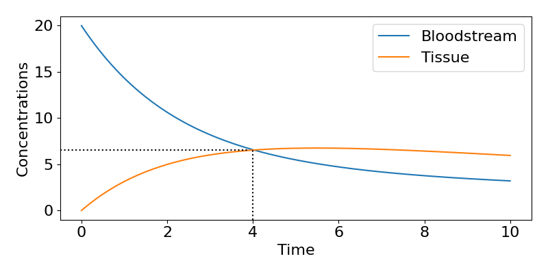
[latex]\begin{equation*} C(t)=20\left[0.75e^{-0.45 t}+0.25e^{-0.05 t}\right]. \end{equation*}[/latex]
All that remains is to substitute in [latex]t=4[/latex] to find that after 4 hours the concentration of the drug will be 6.57mg/L. The plot below shows the full dynamics. It also shows that, purely by chance, 4 hours is roughly the time when the concentrations of the drug in the bloodstream and tissue are equal.
Key Takeaways
- We can extend a model to include more compartments, such as tissues, by having more variables.
- Systems of linear ODEs can be solved to find explicit solutions for each variable.
- With a single dose, the concentrations in all compartments will eventually decay towards zero.
Chapter references
- The content in the Pharmacokinetics section is based on the ebook, Basic Pharmacokinetics by Bourne.
