
6 Diseases of ecological populations
Introduction
In the models of infectious diseases we have covered so far we have been focussing on human populations. However, infectious diseases are also extremely important to the dynamics of many animal, plant and microbial populations (for example, Foot and Mouth, Bovine TB, Wheat Rust, etc.). We should therefore extend our models to consider these cases. There are quite a few changes to our models that we may wish to make so that our models are more reflective of wider ecological populations. Three particular ones we will consider here are:
- We shall now assume that there is no immunity. Hosts can still recover from infection, but they will simply become susceptible once again. (The degree to which even simple organisms possess adaptive immunity is in fact a fascinating question, but for now we will assume it is absent).
- We can no longer reasonably assume that births and deaths are equal.
- We should include the fact that disease causes significant damage to hosts (something we have so far ignored). In particular, we shall assume that infected hosts suffer an additional mortality, or virulence at rate [latex]\alpha[/latex].
Putting these assumptions together with our previous model, we have a new SIS (Susceptible-Infected-Susceptible) model given by,
[latex]\begin{align} &\frac{dS}{dt} = b N - \beta SI - d S + \gamma I\\ &\frac{dI}{dt} = \beta SI - (d+\alpha+\gamma)I. \end{align}[/latex]
A case study: controlling rabbits in Australia
Prior to European settlement, there were no rabbits in Australia (see chapter references). Initially bred for food, their numbers stayed low until a small number were released for hunting purposes on an estate. Within 10 years rabbit numbers were well into the millions.
How might we model this initial population growth? During this early period, we might actually suppose that our very first population growth model provided a good approximation of rabbit dynamics,
[latex]\begin{equation} \frac{dN}{dt} = bN - dN=rN \end{equation}[/latex]
predicting exponential growth for [latex]b\gt d[/latex] (births greater than deaths). We previously criticised this model for not having a carrying capacity, but for populations of rabbits in the hundreds or thousands with the whole continent of Australia to exploit, we might argue that in fact there wasn’t much limiting their growth.
A number of control strategies were attempted through the late 19th- and early 20th-centuries targeting rabbits. In 1950, the myxoma virus was deliberately released in to the rabbit population. From a modelling perspective, the effect of this is to transform the system to the SIS model we introduced above, that is,
[latex]\begin{align} &\frac{dS}{dt} = b N - \beta SI - d S + \gamma I\\ &\frac{dI}{dt} = \beta SI - (d+\alpha+\gamma)I.\\ \end{align}[/latex]
We want to use this model to answer a simple question: will the introduction of the disease successfully control rabbit numbers? Initially we had exponential growth. What we then need to know is whether introducing the disease can limit this growth, perhaps to an equilibrium or even complete eradication.
We can answer this question by analysing our model through our usual methods. First, what are the equilibria of this model? There is an extinction equilibrium at [latex](S,I)=(0,0)[/latex], but this is quickly shown to be always unstable. Also, if [latex]I=0[/latex] then we return to exponential growth of the susceptible rabbit population when [latex]b\gt d[/latex]. But there is also an endemic equilibrium, at,
[latex]\begin{align} S^*&=\frac{d+\alpha+\gamma}{\beta},\\ I^*&=\frac{(b-d)S^* }{\beta S^*-b-\gamma}=\frac{(b-d)(d+\alpha+\gamma)}{\beta(\alpha-(b-d))}. \end{align}[/latex]
To determine whether this equilibrium is stable, and so whether the disease can indeed control the rabbit population to this equilibrium level, we need to look at the Jacobian.
Exercises
Write out the general Jacobian for this system.
Click for solution
Taking the partial derivatives of the ODEs and putting them in the Jacobian matrix we get,
[latex]\begin{align*} J=&\left( \begin{array}{cc} b-d-\beta I^* & b-\beta S^*+\gamma\\ \beta I^* & \beta S^*-(\alpha+d+\gamma) \end{array} \right). \end{align*}[/latex]
Substituting in our equilibrium values for [latex]S^*[/latex] and [latex]I^*[/latex] we find that,
[latex]\begin{align} J=&\left( \begin{array}{cc} b-d-\frac{(b-d)(d+\alpha+\gamma)}{(\alpha-(b-d))} & b-d-\alpha\\ \frac{(b-d)(d+\alpha+\gamma)}{(\alpha-(b-d))} & 0 \end{array} \right) \end{align}[/latex]
From here we can find that [latex]\det=(b-d)(d+\alpha+\gamma)[/latex], which is positive provided [latex]b\gt d[/latex]. Stability will therefore depend on the trace. With some re-arranging, we have [latex]tr=(b-d)(b+\gamma)/[(b-d)-\alpha][/latex]. Since we are assuming [latex]b\gt d[/latex] then the numerator is positive. For the fixed point to be stable we require [latex]tr\lt 0[/latex] which therefore requires [latex]\alpha>(b-d)[/latex] in the denominator. So, if the rate of virulence (infection-induced mortality) is greater than the rate of intrinsic population growth, the endemic equilibrium is stable. Otherwise it is unstable and we would expect exponential growth.
So, what can we conclude here? That for an exponentially growing population of rabbits, provided the disease is sufficiently virulent, introducing the myxoma virus will control the rabbit population to an equilibrium level. We have therefore shown that an infectious disease can be used as an effective control mechanism against biological invasions.
A free-living parasite model
There are even more different additional assumptions we may look to include in a model representing infectious disease spread in wildlife populations. We’ll now look at a case where we assume that infection is not simply through direct contact between susceptible and infected hosts, but where the parasite is free-living in the environment, and infection occurs when susceptible hosts pick up these free-living stages. Letting [latex]P[/latex] be the density of free-living parasites, one way to model this would be as follows,
[latex]\begin{align} &\frac{dS}{dt} = bS-dS-\beta SP\\ &\frac{dI}{dt} = \beta SP - (d+\alpha)I\\ &\frac{dP}{dt}=\phi I-\mu P. \end{align}[/latex]
The key differences to our previous models are:
- The transmission term [latex]\beta SP[/latex] now requires contact between susceptible hosts and free-living parasite stages for infection to occur.
- Free-living parasites are produced at a constant rate by infected hosts.
- Free-living parasites die at rate [latex]\mu[/latex], and we assume the loss of parasites due to infection can be ignored.
As ever with modelling, many of these processes could be formed differently or have different underlying assumptions, but this gives us a model we can work with.
What equilibria does this model give us? We will have a trivial equilibrium of nothing present, and since we again do not include density-dependence in the susceptible host’s dynamics we will not have a disease-free equilibrium (if the parasite is not present, meaning [latex]I=P=0[/latex], then the host population increases without bound). This just leaves an endemic equilibrium.
Exercises
Click for solution
Using the first ODE we can take out [latex]X[/latex] as a factor, which tells us,
[latex]\begin{align} a-b-\beta P&=0\\ \implies P^*&=\frac{a-b}{\beta}. \end{align}[/latex]
Then from the third ODE we have,
[latex]\begin{align} \phi I&=\mu P\\ \implies I^*&=\frac{\mu P^*}{\phi}\\ \implies I^*&=\frac{\mu (a-b)}{\phi\beta} \end{align}[/latex]
Finally we use the second ODE to find an expression for [latex]S^*[/latex],
[latex]\begin{align} \beta SP-(\alpha+b)I&=0\\ \implies S^*&=\frac{(\alpha+b)I^*}{\beta P^*}\\ \implies S^*&=\frac{(\alpha+b)\mu}{\phi\beta}. \end{align}[/latex]
What can we say about stability here? We still need to use the Jacobian to assess stability, but it is now a 3×3 matrix,
[latex]\begin{align*} J=&\left( \begin{array}{ccc} 0 & 0 & -\beta S^*\\ \beta P^* & -\alpha-b & \beta S^*\\ 0 & \phi & -\mu \end{array} \right). \end{align*}[/latex]
We have not covered how to assess stability in a three-dimensional system in any case so far but you can read about it in the background review chapter on linear stability analysis. As a brief summary here, the general rule for stability is that if all the eigenvalues from the Jacobian matrix are negative an equilibrium is stable, and if any eigenvalues are positive the equilibrium is unstable (or a saddle). We have seen that for two-dimensional systems we can sometimes find these eigenavlues directly, and in more complicated cases we use the trace-determinant condition. In fact, this latter condition is a special case of stability criteria called Routh-Hurwitz conditions. This is what we need to use here. Often this can be very messy and hard to get meaningful results out of, but sometimes we are lucky and things fall out easily. This case is … in-between.
Firstly we write out the characteristic equation given by [latex]\det(J-\lambda I_3)=0[/latex] where [latex]I_3[/latex] is the 3×3 identitiy matrix. This gives,
[latex]\begin{equation} \det(J-\lambda I_3)=\lambda\left[(\alpha+b+\lambda)(\mu+\lambda)-\beta S^*\phi\right]+\beta S^*\beta P^*\phi=0. \end{equation}[/latex]
To use the Routh-Hurwitz criteria we need to write this out in the form [latex]\lambda^3+a_2\lambda^2+a_1\lambda+a_0[/latex]. For our equation this gives,
[latex]\begin{align} \det(J-\lambda I_3)=&\lambda^3+\\ &\lambda^2[\alpha+b+\mu]+\\ &\lambda [(\alpha+b)\mu-\beta S^*\phi]+\\ &\beta S^*\beta P^*\phi=0. \end{align}[/latex]
The Routh-Hurwitz criteria tell us that for a 3×3 system, stability requires, [latex]a_2,a_1,a_0\gt0[/latex] and [latex]a_2a_1\gt a_0[/latex]. Looking at our equation, we can see that [latex]a_2[/latex] and [latex]a_0[/latex] are definitely positive. However, if we substitute in the value for [latex]S^*[/latex] we find that [latex]a_1=0[/latex]. This same result also means that we never satsify [latex]a_2a_1\gt a_0[/latex], meaning that this equilibrium is never stable.
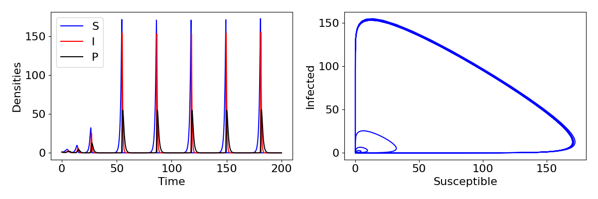
So if the endemic equilibrium is never stable, what does happen in this system? It would be surprising if the disease never persisted and we only ever had exponential growth of hosts. It is difficult to prove mathematically, but the answer is that the system exhibits limit cycles (like we saw in the predator-prey model). An example of these cycles are shown in the plot below, showing really quite sharp and extreme cycles, with rapid outbreaks of infection followed by collapse to near-extinction. This change occurs because the free-living parasite has introduced a delay to the infection process. The rate of infection experienced by a susceptible no longer depends on the current infected density but on what that density was a few time-steps ago when it was producing the free-living stages. In general, introducing delays into models has the tendency to cause cycles.
Explore the model
Use the Python code below to explore the free-living parasite model. This will produce plots of the time-courses and a phase-portrait for [latex]S[/latex] and [latex]I[/latex], showing very large cycles. Using the parameter values, calculate what the equilibrium values would be – how much larger do the densities grow on the cycles than the equilibria? Try changing a few parameters to see how the nature of the cycles change.
You may well find that if you change parameter values the model begins to run slowly or even stops entirely and sends an error message. This is an example of a stiff ODE system. Roughly, this is a system where the dynamics have two very different time-scales – for example in this case the dynamics spend a good deal of time with densities close to 0 and not changing, followed by very rapid increases – and standard numerical ODE solvers often struggle to run such models. Approaches to overcome this include using an alternative solver (you can add the optional argument, method='Radau' to the end of the solve_ivp function to do this here) or log-transforming the model to take new variables [latex]\bar{S}=\ln{S}[/latex], etc, and solving for the transformed model of [latex]d\bar{S}/dt[/latex], etc.
Click for code
# Import the necessary librariesimport numpy as npimport matplotlib.pyplot as pltfrom scipy.integrate import solve_ivp# Options to make the plots the right sizeplt.rcParams['figure.figsize'] = [12, 4]plt.rcParams.update({'font.size': 16})# Function for dynamics called 'freeliving'def freeliving(t,x): # Rename variables for ease S=x[0] I=x[1] P=x[2] # The ODEs dS = a*S-b*S-beta*S*P dI = beta*S*P-(alpha+b)*I dP = phi*I-mu*P return [dS,dI,dP]# Parameter valuesa=2b=1alpha=1mu=1beta=1phi=1# Initial conditionsS0=1I0=1P0=1N0=[S0,I0,P0]# Time points to usetc = np.linspace(0, 200, 10000)
# Run model using 'solve_ivp'Nc = solve_ivp(freeliving, [tc[0],tc[-1]],N0, t_eval=tc)# Plotting codefig, (ax1, ax2) = plt.subplots(1, 2)ax1.plot(tc, Nc.y[0], "r", label="S") ax1.plot(tc, Nc.y[1], "k", label="I")ax1.plot(tc, Nc.y[2], "b", label="P")ax1.set(xlabel='Time', ylabel='Concentrations')ax1.legend()ax2.plot(Nc.y[0],Nc.y[1],'b')ax2.set(xlabel='S', ylabel='I')Key Takeaways
- If we model disease in ecological populations we need to make some changes to our model, for example including disease-induced deaths.
- If a disease is sufficiently deadly, it can be used as a biological control of a pest species.
- If disease is caused by a free-living paraiste stage, this can lead to cycles of infection.
Chapter references
- The rabbit-myxoma model is based on an example in a paper by Anderson and May (1982).
- The free-living parasite model is based on an example in the paper by Anderson and May (1981).
- The content in the Infectious diseases section was influenced by the textbooks, Mathematical Biology by Murray and Modelling Infectious Diseases in Humans and Animals by Keeling & Rohani.
