Introducing bifurcations

In most of the models in this textbook we find that we can get a number of qualitatively different outcomes depending on the parameters. Very often we find that equilibria and their stability vary as we change different parameters, and specific values where equilibria collide, appear and change stability. These are important transitions known as bifurcations and are one of the most important aspects of a dynamical system. Bifurcations tell you when and how you can expect discrete shifts in behaviour as you change one or more parameters.

There are only a few different types of bifurcation that are possible, and we will cover the fundamental ones here. In all cases we will see how changing a particular parameter leads to a change in the stability, or existence of, the equilibria in the model. We will largely do this by looking at bifurcation diagrams. These plot the location and stability (solid lines denote stable equilibria, dashed lines unstable) of equilibria as parameters vary.

The first three examples can all be seen in one-dimensional (i.e. one variable) models as well as in higher dimensions. (There is some formal mathematical work and terminology behind bifurcations that we will not concern ourselves with here. If you want to know more, the textbook Nonlinear Dynamics and Chaos, by Strogatz is a very good place to start.)

Standard bifurcations

Transcritical bifrucation

The transcritical bifurcation is perhaps the most common form of bifurcation in a mathematical biology model. It occurs when two equilibria intersect and swap stability. It is so common because we will usually have a trivial equilibrium where nothing exists, which will lose stability when it intersects with an equilibrium where something exists.

An example is shown in the diagram below (which is actually from the spruce budworm model in chapter 1). For [latex]\rho\lt100[/latex] the [latex]N=0[/latex] equilibria is unstable. Technically a second equilbiria exists at [latex]N0[/latex], which would be locally stable, but is not biologically feasible. For [latex]\rho\gt100[/latex] we see that now the [latex]N=0[/latex] equilibrium is stable, with the second equilibrium now present at [latex]N>0[/latex] being unstable. The point where these two equilibria meet and swap stability, [latex]\rho=100[/latex] is the transcriticial bifurcation.

Saddle-Node bifurcation

The transcritical bifurcation occurs when (at least) one equilibria exists over a large range of the parameter (i.e. the trivial equilibrium). However, there are also cases where equilibria can be created or destroyed as a parameter is varied. These are called saddle-node or blue-sky bifurcations (the former because what gets created at the bifurcation is a stable-unstable pair of equilibria; the latter because the equilibria appear out of the clear blue sky)

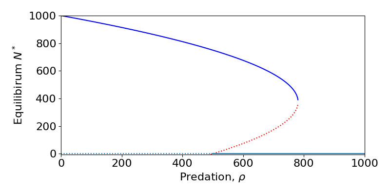
An example of a saddle-node bifurcation can again be seen from the spruce budworm model. For $latex\ rho\gt300$ we see that only the [latex]N=0[/latex] equilibrium exists. As [latex]\rho[/latex] is reduced the two non-zero equilibria appear, one stable and the other a saddle, and diverge.

Saddle-node bifurcations thus have very important consequences for any biological system. It means that there may not be a gradual and steady decrease down to extinction (as in the transcritical case), but a very sudden crash. This is often termed ‘a catastrophe’ and is a focus of much research to understand the risk of sudden extinctions in real populations. For example, models of fisheries management show that if the rate of fishing becomes too high we may see sudden declines in fish stocks. Moreover, the decline is very hard to reverse as a small decrease in the harvesting rate does not easily return the system to the stable equilibrium as the saddle is still pushing the population densities lower. This is an example of hysteresis.

Pitchfork bifurcation

The third type of standard bifurcation – the pitchfork – does not occur in any of the models covered in this textbook (it is usually a result of strong symmetry in a system). However, for completeness we shall briefly mention it here.

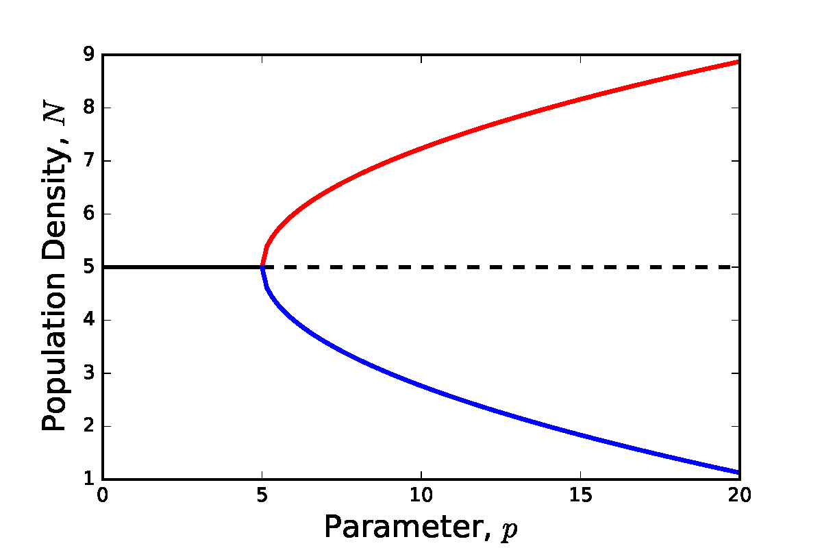
The reason for the naming of this bifurcation is obvious by looking at the bifurcation diagram below. At low value of the bifurcation parameter there is a single stable equilibria. At the bifurcation point this existing point remains but loses stability, and two new stable equilibria emerge.

Hopf Bifurcation

The final type of bifurcation we will cover here is only seen in systems of two or more dimensions. A Hopf bifurcation occurs when varying a parameter alters an equilibrium that was a stable spiral into an unstable spiral (or vice versa). This is a particularly important behaviour, because as we initially move into the unstable spiral a unique, stable closed orbit emerges from the equilibrium, resulting in the population cycling/oscillating. It is not very easy to draw a bifurcation diagram in this case, but we can usually see the process by looking at the phase portraits as we vary a parameter and seeing how the limit cycle emerges. Examples of this are seen in chapters 3 and 15.