A model for Covid-19

In the last few chapters we were thinking about the dynamics of disease at the scale of human or ecological populations. Often, though, we will be more concerned with the health of individual patients, particularly from a medical perspective. In these cases, we want to know how a virus or bacteria grows and develops inside the body, and how our immune system interacts with it. To study these dynamics we therefore require a within-host model. As we move down in biological scales, for the biology novice some of the terminology and ideas will now start to feel less familiar, but it is important to remember that we are still dealing with populations. But whereas we previously thought of populations as groups of humans or animals, we are now looking at populations of cells or virus particles.

In our first example we will look at a relatively simple model of virus-cell dynamics that loosely describes the interaction between Covid-19 virus particles and a type of human immune cell called the T-cell (see chapter references). We assume that the virus grows in the body according to classic logistic growth that we met back in the first chapter, that it decays at some background rate, but that it is also killed by T-cells. T-cells themselves are produced by the body at some constant, background rate, but also proliferate when they sense virus is present. Finally the T-cells also decay. We can write down our model as follows,

[latex]\begin{align} \frac{dV}{dt} &= pV(1-V/K)-\beta VT - \mu V\\ \frac{dT}{dt} &= s+rT\left(\frac{V^2}{V^2+c^2}\right)-\delta T \end{align}[/latex]

As usual, all the parameters are positive and we will also assume that [latex]r>\delta[/latex]. There are a few things to notice about this model:

• When a virus is killed by a T-cell, there is no corresponding killing of the cell itself.
• T-cell production is constant, not a per-capita rate.
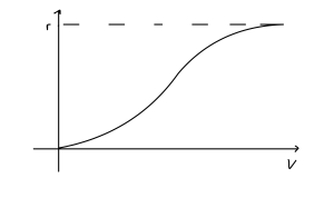
• The proliferation function is sigmoidal – while virus density is small little proliferation occurs, but past a threshold value it rapidly increases. Quite a lot of the analysis is going to depend on knowledge of what this proliferation function looks like.

As you will be getting used to, we will first consider the equilibria of this system. If we factorise the first equation we find two possible ways to make it equal zero:

• [latex]V=0[/latex]
• [latex]p(1-V/K)-\beta T - \mu =0 \implies T=(p(1-V/K)-\mu)/\beta[/latex]

Substituting [latex]V=0[/latex] into the second equation, we can find that this requires [latex]T=s/\delta[/latex] for an equilibrium. This will be the virus-free equilibrium, with no virus and T-cells present at their background density.

For the second equilibrium we can see that the result of making the substitution of [latex]T[/latex] into our second ODE is likely to leave something quite complicated. Indeed, there may even be more than one equilibrium produced. To save ourselves a lot of tedious algebra let us instead examine the phase portrait.

A graphical analysis

We have a two-dimensional system and both variables must be non-negative to make biological sense. We can use the workings we used when finding the equilibria to help us find the nullclines. The nullclines from the first equation give us:

• [latex]V=0[/latex] – a straight vertical line.
• [latex]T=p(1-V/K)-\mu)/\beta[/latex] – a decreasing straight line starting at [latex](p-\mu)/\beta[/latex] and crossing 0 at [latex]V=K(1-\mu/\beta)[/latex].

After a couple of lines of working we can find the single nullcline from the second equation to be,

• [latex]T=\frac{s}{\delta-r\left(\frac{V^2}{V^2+c^2}\right)}[/latex].

What does this nullcline look like? It starts at [latex]T=s/\delta[/latex] when [latex]V=0[/latex] and as [latex]V[/latex] gets very large we find [latex]T\to s/(\delta-r)[/latex]. In between these extremes we have this sigmoidal proliferation function to worry about. Note that [latex]V^2/(V^2+c^2)[/latex] varies from 0 to 1 and is strictly increasing and that [latex]r\gt\delta[/latex]. This tells us two things:

1. The nullcline is strictly increasing.
2. At some point the denominator will pass through zero (some further work finds that techncially this happens twice, but one of the values occurs for [latex]V\lt0[/latex]). After this happens we will have [latex]T\lt0[/latex].

One additional thing to note is that the term, [latex]V^2/(V^2+c^2)[/latex] remains small up to reasonably high values of [latex]V[/latex]. Therefore this term will initially not effect the nullcline much as [latex]V[/latex] increases, meaning our nullcline is initially quite flat. We can put all of this together to form our phase portrait.

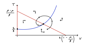
What we see, then, is that there is only one equilibrium when the virus is present, and for the assumptions we have made about relative parameter values, it appears to be a stable spiral. We can additionally note that the initial dynamics are for a rapid rise in virus concentration but little change in T-cell density, before the virus becomes more prevalent and T-cell proliferation begins. We can also note that the virus density at the equilibrium is considerably lower than it would be without T-cells doing their thing. Examining the phase portrait, we might also conclude that the virus-free equilibrium will only become stable if we can move the [latex]T[/latex] nullcline far enough upwards that the two non-zero nullclines no longer intersect. This would require [latex]s/\delta\gt(p-\mu)/\beta[/latex]. Let us see if we can confirm that conclusion with linear stability analysis.

Linear stability analysis

The general Jacobian for the system is given by,

[latex]\begin{align*} J=&\left( \begin{array}{cc} p-\frac{2pV^*}{K}-\beta T^*-\mu & -\beta V^*\\ rT^*\frac{2V^*c^2}{(V^{*2}+c^2)^2} & r\frac{V^{*2}}{V^{*2}+c^2}-\delta \end{array} \right) \end{align*}[/latex]

Virus-free equilibrium

Since [latex]V^*=0[/latex] both the top-right and bottom-left entries are zero, meaning we can read off the eigenvalues as the two terms on the main diagonal:

• [latex]\lambda_1=p-\beta T^*-\mu[/latex]
• [latex]\lambda_2=-\delta[/latex]

The second eigenvalue is negative, so everything depends on the first. Re-arranging we require [latex]T^*>(p-\mu)/\beta[/latex]. Recall that for the virus free equilibrium we have [latex]T^*=s/\delta[/latex]. Therefore this equilibrium is only stable when [latex]s/\delta>(p-\mu)/\beta[/latex], exactly as we surmised was the case from our phase portrait.

Virus-present equilibrium

You will recall that we never wrote down an expression for this equilibrium. You might remember from previous chapters, however, that this does not usually stop us making conclusions about its stability. We know from the phase portrait that there is only one equilibrium to worry about. We also know from the equilibrium conditions that:

• [latex]p(1-V^*/K)-\beta T-\mu=0[/latex]
• [latex]rV^{*2}/(V^{*2}+c^2)-\delta = -s/T^*[/latex].

Substituting these values in to the Jacobian we now find,

[latex]\begin{align*} J=&\left( \begin{array}{cc} -\frac{pV^*}{K} & -\beta V^*\\ rT^*\frac{2V^*c^2}{(V^{*2}+c^2)^2} & -s/T^* \end{array} \right) \end{align*}[/latex]

Now we must assess stability based on the trade and determinant conditions. These are:

[latex]tr(J)=-\frac{pV^*}{K}-\frac{s}{T^*} \lt 0[/latex]

[latex]\det(J)=\frac{psV^*}{KT^*}+r\beta V^*T^*\left(\frac{2V^*c^2}{V*^2+c^2}\right)\gt 0[/latex]

This means that whenever the equilibrium at [latex]V^*,T^*\gt0[/latex] exists, it must be stable. And we know from the phase portrait that the condition for it to exist is the exact opposite of the condition for stability of the virus-free equilibrium.

Chapter references

• This chapter is based on a model from Hernandez-Vargas & Velasco-Hernandez (2020).