Why repeated doses might be a problem

In our first pharmacokinetic model we assumed that only one dose of the drug was given to the patient, and then thought about how its concentration decayed over time. In certain circumstances this may well be all that happens – for example you may often have taken one dose of paracetamol for a headache. However, for ongoing, chronic conditions, a patient will take repeated doses of a drug. This leads to an important question: what is the optimal dosage and time interval between doses for a particular drug? We would certainly like to ensure the patient always has a minimal amount of the drug in their system so that it is always being effective. However, we also need to ensure the patient never has too much drug in their system, avoiding overdoses.

There is a potential problem, though. In the previous model we could assume that we started with no drug in the bloodstream. After repeated doses, however, the drug will accumulate. Even if we wait a very long time for the 2nd dose, there will still be some small amount of the 1st dose left. That means that when we add on the new dose we will end up with a greater concentration than we had initially. If this keeps on adding up, there is a danger we will eventually reach dangerous levels of the drug in the bloodstream. Let’s try and figure out if this really will be a problem by considering an example.

Click for solution

Dose no.	Concentration after dose	Concentration before dose
1	4	2
2	6	3
3	7	3.5
4	7.5	3.75

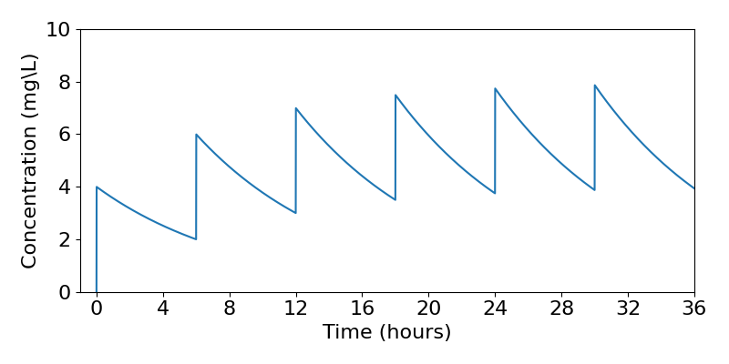
The concentrations for the first four doses are shown in the table above. A full time course of the concentrations is shown in the plot below. Eventually the concentrations of the drug simply fluctuate between 8mg/L and 4mg/L. There is thus a limit to accumulation, because eventually the constant amount being added becomes equal to the density-dependent amount being removed. It therefore looks like we could design our drug dosage regime to safely oscillate between some finite maximum and minimum concentrations.

Mathematical derivation

As a good scientist, you should always be sceptical of being presented with one case. Will repeated doses always balance out in the end like this? Or have I been sneaky in presenting a unique example to you? To check this, the key is to spot that in fact this process is given by a geometric series. Recall from our first model that if the dynamics of the drug are given by,

[latex]\begin{equation} \frac{dC}{dt} =-kC, \end{equation}[/latex]

then,
[latex]\begin{equation} C(t)=C_0e^{-kt}. \end{equation}[/latex]

Suppose that we give a dose of the drug every [latex]\tau[/latex] hours. We will also label the concentrations with a subscript to denote which number dose we are considering. Thus [latex]\tau[/latex] hours after the first dose, but immediately before the second dose, we have,

[latex]\begin{equation} C_1(\tau)=C_0e^{-k\tau}. \end{equation}[/latex]

The second dose is then administered. Immediately after this second dose (re-starting ‘time since last dose’ as [latex]t=0[/latex]) we have,

[latex]\begin{equation} C_2(0)=C_1(\tau)+C_0=C_0(1+e^{-k\tau}). \end{equation}[/latex]

This quantity is therefore the new initial condition, and the dynamics for the next [latex]\tau[/latex] hours will now be given by,

[latex]\begin{equation} C_2(t)=C_0(1+e^{-k\tau})e^{-kt}, \end{equation}[/latex]

and exactly [latex]\tau[/latex] hours after this second dose, but just before the third,

[latex]\begin{equation} C_2(\tau)=C_0(1+e^{-k\tau})e^{-k\tau}. \end{equation}[/latex]

This pattern continues. For example immediately after and [latex]\tau[/latex] hours after the third dose we have, respectively,

[latex]\begin{align} C_3(0)&=C_0(1+e^{-k\tau})e^{-k\tau}+C_0=C_0(1+e^{-k\tau}+e^{-2k\tau}),\\ C_3(\tau)&=C_0(1+e^{-k\tau}+e^{-2k\tau})e^{-k\tau}. \end{align}[/latex]

This is beginning to look a little messy. To help matters, let [latex]R=e^{-k\tau}[/latex]. Then we can re-write these two expressions as,

[latex]\begin{align} C_3(0)&=C_0(1+R+R^2),\\ C_3(\tau)&=C_0(R+R^2+R^3). \end{align}[/latex]

From here we can extrapolate to the concentrations after the [latex]n[/latex]-th dose,

[latex]\begin{align} C_n(0)&=C_0(1+R+R^2+...+R^{n-1})=\sum_{i=1}^{n}C_0R^{n-1},\\ C_n(\tau)&=C_0(R+R^2+R^3+...R^n)=\sum_{i=1}^{n}C_0R^{n}. \end{align}[/latex]

These are geometric series! A nice property of such series is that we can express this as a simple fraction as follows,

[latex]\begin{align*} C_n(0)&=C_0(1+R+R^2+...+R^{n-1})\\ RC_n(0)&=C_0(R+R^2+...+R^n)\\ C_n(0)-RC_n(0)&=C_0(1-R^n)\\ C_n(0)&=C_0\frac{1-R^n}{1-R}=C_0\frac{1-e^{-nk\tau}}{1-e^{-k\tau}}. \end{align*}[/latex]

By similar reasoning we can find that,

[latex]\begin{equation} C_n(\tau)=C_0R\frac{1-R^n}{1-R}=C_0e^{-k\tau}\frac{1-e^{-nk\tau}}{1-e^{-k\tau}}. \end{equation}[/latex]

This also leads to an equation for the concentration at any time, [latex]t[/latex], after the [latex]n[/latex]-th dose,

[latex]\begin{equation} C_n(t)=C_0e^{-kt}\frac{1-e^{-nk\tau}}{1-e^{-k\tau}}. \end{equation}[/latex]

We can then look at what happens in the long-term by letting [latex]n\to\infty[/latex] to find the minimum and maximum concentrations of the drug after many doses. Because we know that [latex]e^{-k\tau}\lt1[/latex], we can say that [latex]e^{-nk\tau}\to0[/latex] as [latex]n\to\infty[/latex], meaning we have,

[latex]\begin{equation*} C_{\infty}(0)=C_+=\frac{C_0}{1-e^{-k\tau}} \end{equation*}[/latex]

for the maximum concentration, and,

[latex]\begin{equation*} C_{\infty}(\tau)=C_-=\frac{C_0e^{-k\tau}}{1-e^{-k\tau}} \end{equation*}[/latex]

for the minimum.

Notice that this approach works so long as [latex]e^{-k\tau}\lt1[/latex], but this is always true for the biologically realistic assumptions that [latex]k,\tau\gt0[/latex]. So we will always reach finite maxima and minima that the concentration fluctuates between.

Designing a drug dosage regime

In that last exercise you were told a dose amount and time interval, calculated the (long-term) maximum and minimum concentrations, and then checked back to see if they fitted some given guidelines. Now let’s think about the problem a different way. Suppose we wish to design our dosage regime so that it fits the clinical guidelines exactly – that is a maximum concentration of 20mg/L and a minimum of 7.5mg/L. What should the dosage amount and time interval be? We already know that [latex]k=0.154[/latex]. First, notice that,

[latex]\begin{align*} \frac{C_{\infty}(\tau)}{C_{\infty}(0)}&=R=e^{-k\tau}\\ \implies\frac{7.5}{20}&=e^{-0.154\tau}. \end{align*}[/latex]

By taking logs and re-arranging this we get [latex]\tau=-\ln(0.375)/0.154=6.369[/latex]h. Let’s round this to the more realistic time frame of 6 hours.

Then by considering the maximum we have,

[latex]\begin{align*} C_0&=C_{\infty}(0)(1-e^{-k\tau})\\ \implies C_0&={20}{(1-e^{-0.154\times6})}\\ \implies C_0&=12.061\textrm{mg/L}. \end{align*}[/latex]

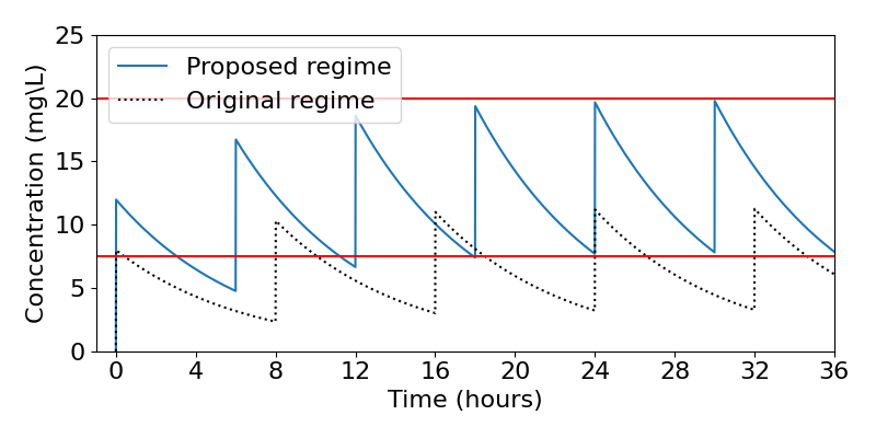
Given that [latex]V=25[/latex], this means a dose of 301.525mg, which we might round down (because we definitely wish to avoid overdosing) to the more realistic 300mg. Thus, based on our knowledge of the drug, we would recommend a dose of 300mg every 6 hours for maximum, yet safe, efficacy. (A quick check shows that our rounding means this actually gives a maximum of 19.90mg/L and a minimum of 7.90mg/L.) A time course of this proposed regime is shown in the figure below, along with the original regime which we can see was much less efficient.

Loading dose and maintenance dose

A downside of the approach we have just described is that it might take a long time for the drug concentration to reach these long-term maximum and minimum values. What we might consider doing, then, is to initiate treatment with a larger loading dose that takes the concentration to (or near) the maximum concentration, with following dosages given as a maintenance dose. The loading dose should come as close as possible to immediately reaching the maximum concentration. For our example above, then, we might take a loading dose of [latex]20\times25=500[/latex]mg. The maintenance dose and timing would then be identical to previously (300mg every 6 hours) since this regime is already balanced to fluctuate between the maximum and minimum concentrations.

We can still write a general solution by considering the dynamics over subsequent doses. Calling the loading dose [latex]C_L[/latex] and the maintenance dose [latex]C_M[/latex], some time [latex]t[/latex] after the fist dose we have,

[latex]\begin{equation} C_1(t)=C_Le^{-kt}. \end{equation}[/latex]

Immediately after the second dose at time [latex]\tau[/latex], re-starting time as [latex]t=0[/latex], we have,

[latex]\begin{equation} C_2(0)=C_1(\tau)+C_M=C_M+C_Le^{-k\tau}, \end{equation}[/latex]

and the dynamics for the next [latex]\tau[/latex] hours will now be given by,

[latex]\begin{equation} C_2(t)=[C_M+C_Le^{-k\tau}]e^{-kt}. \end{equation}[/latex]

Then, immediately after the third dose we have,

[latex]\begin{equation} C_3(0)=C_M+[C_Me^{-k\tau}+C_Le^{-2k\tau}]. \end{equation}[/latex]

Note that we can then re-write this as,

[latex]\begin{equation} C_3(0)=C_M[1+e^{-k\tau}+e^{-2k\tau}]+(C_L-C_M)e^{-2k\tau}. \end{equation}[/latex]

and for any time [latex]t[/latex] after this we would have,

[latex]\begin{equation} C_3(t)=C_M[1+e^{-k\tau}+e^{-2k\tau}]e^{-kt}+(C_L-C_M)e^{-2k\tau}e^{-kt}. \end{equation}[/latex]

We can see the first term is exactly the same as we had previously and will again be given by a geometric sum. There is then the addition of a second term to do with the extra loading dose. The final expression for the dynamics in this case are thus given by,

[latex]\begin{equation} C_n(t)=C_Me^{-kt}\frac{1-e^{-nk\tau}}{1-e^{-k\tau}}+(C_L-C_M)e^{-k[(n-1)\tau+t]}. \end{equation}[/latex]

Chapter references

• The content in the Pharmacokinetics section is based on the ebook, Basic Pharmacokinetics by Bourne.