Case study: Red and grey squirrels

Populations rarely (if ever) exist in isolation. In reality, the growth rate of a given population depends not only on itself, but also on other populations that it interacts with either directly or indirectly. Such interactions lead to a range of ecological relationships, including competition for resources, predation, mutualism, parasitism and more besides. In the next chapters we will study models that represent a few of these different interactions.

Our first example will be of two species that compete for a common resource. This is sometimes known as the Lotka-Volterra model (though I personally try to avoid using labels named after people – they can be confusing and ingrain bias) or interspecific competition. To guide our thinking we will have a case study in mind, namely red and grey squirrels – well-known competitors in the UK – but we could equally consider microbes competing for substrates, plants competing for water or nutrients or a whole host of species competing with one another for territory or food. As with our previous single population models, we begin by considering what factors might contribute to the birth and death mechanisms that control the rates of changes of the two populations. We will assume:

• There is only a limited supply of food for squirrels to eat. This means that even in the absence of interspecific competition, the environment would have a limited carrying capacity (i.e. a maximum number of squirrels that it could support). The population dynamics for each species on its own can be modelled using a logistic growth equation (that does include intraspecific competition between individuals in the same population).
• The effect of one species on the other is proportional to its population size (since the more there are, the less food, territory and other resources will be available). Therefore there will be a term in each equation causing a reduction in growth that is given by the product of the two species’ densities.

We also assume that the carrying capacity for the two species of squirrel can be different (perhaps because one species can eat a wider variety of food than the other), and that the two species can have different susceptibilities to competition (perhaps because one species is more timid than the other). Without interspecific competition, we could model the two populations using two logistic growth equations:

[latex]\begin{align} \frac{dR}{dt} & =R(a-R) \\ \frac{dG}{dt} & =G(c-G), \end{align}[/latex]

where [latex]R[/latex] and [latex]G[/latex] represent the respective population densities of red and grey squirrels. Note that we have already done a little non-dimensionalising here, and that [latex]a[/latex] and [latex]c[/latex] are thus the respective carrying capacities (since if, for example, [latex]R\gt a[/latex], we have [latex]dR/dt\lt 0[/latex]). To include competition between the species, we add an additional term to each equation:

[latex]\begin{align} \frac{dR}{dt} & =R(a-R-bG) \\ \frac{dG}{dt} & =G(c-dR-G), \end{align}[/latex]

where [latex]b[/latex] and [latex]d[/latex] are the strengths of interspecific competition. While this model is only a little more complicated than the logistic model, this system cannot be solved explicitly since it is non-linear. We will therefore need to take a qualitative approach to understanding what can possibly happen in this model. However, we can still gain considerable insight in to the system by applying the tools of dynamical systems. See the appropriate background review chapters on phase portraits and linear stability analysis if needed.

Analysis

Phase portraits

A good way to visualise what is happening here is through a phase portrait. As discussed in more detail in the background review chapter, our phase portrait can be built up using the following procedure:

1. Draw axes of the two key variables.
2. Determine how much of the phase plane is biologically feasible.
3. Calculate nullclines and draw them on your plot.
4. Mark on equilibria where two (different) nullclines cross.
5. Work out the qualitative directions of travel in each of the regions separated by the nullclines and draw arrows on your phase portrait to show these direction fields.
6. Optionally use linear stability analysis to get a clearer picture of behaviour around the equilibria.
7. Sketch on some sample trajectories.

In this example our two axes will be our population densities, [latex]R[/latex] and [latex]G[/latex], and we know both densities must be non-negative. Now let us find the nullclines:

[latex]\begin{align*} &\frac{dR}{dt}=0 \implies R=0 \quad \mathrm{ or } \quad G=\frac{a-R}{b}\\ &\frac{dG}{dt}=0 \implies G=0 \quad \mathrm{ or }\quad G=c-dR \end{align*}[/latex]

We therefore have a nullcline along each axis, and two nullclines which are decreasing straight lines on our plot. Qualitatively, there are four different ways we can configure these two nullclines:

1. Red starts above Grey and they do not cross (in the biologically feasible region).
2. Grey starts above Red and they do not cross (in the biologically feasible region).
3. Grey starts above Red and they do cross.
4. Red starts above Grey and they do cross.

When drawing the direction fields we can say that,

• If [latex]R[/latex] and [latex]G[/latex] are both small (we are below both nullclines), [latex]dR/dt\gt 0[/latex] and [latex]dG/dt\gt 0[/latex].
• If [latex]R[/latex] and [latex]G[/latex] are both large (we are above both nullclines), [latex]dR/dt\lt 0[/latex] and [latex]dG/dt\lt 0[/latex].
• If we are above the [latex]R[/latex]-nullcline but below the [latex]G[/latex]-nullcline, [latex]dR/dt\lt 0[/latex] but [latex]dG/dt\gt 0[/latex].
• If we are below the [latex]R[/latex]-nullcline but above the [latex]G[/latex]-nullcline, [latex]dR/dt\gt 0[/latex] but [latex]dG/dt\lt 0[/latex].

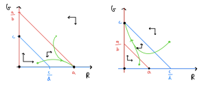
This gives us enough information to sketch out the four phase portraits and assess the qualitative behaviour. The first two cases that we listed above are sketched out below. Work your way through the procedure above and see how these have been built up.

Click for solution

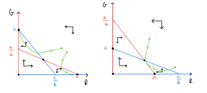
The remaining two phase portraits should look like this:

Let’s consider what these phase portraits show. Firstly, what are the possible equilibria? We see that equilibria at [latex](0,0)[/latex], [latex](a,0)[/latex] and [latex](0,c)[/latex] are always present (an [latex]R[/latex]-nullcine and [latex]G[/latex]-nullcline always cross at these values). These respectively mean no squirrels present, only red squirrels present and only grey squirrels present. Then we sometimes have another equilibrium – if [latex]a\gt bc[/latex] and [latex]c\gt ad[/latex] or [latex]a\lt bc[/latex] and [latex]c\lt ad[/latex] – where both species are present.

Which of these equilibria would we end up going to in each case? Looking through our four phase portraits in turn we find,

1. [latex]R[/latex] “wins” and settles to a steady population level, while [latex]G[/latex] goes extinct.
2. [latex]G[/latex] “wins” and settles to a steady population level, while [latex]R[/latex] goes extinct.
3. The outcome depends on the starting condition, with either [latex]R[/latex] or [latex]G[/latex] eventually winning out and sending the other population to extinction.
4. [latex]R[/latex] and [latex]G[/latex] co-exist at steady non-zero population levels.

We have therefore sketched out all the possible outcomes in a competition model without finding explicit solutions for the two populations (remember, such solutions do not even exist). We can see that in theory two species can coexist, but it requires a particular balance of competition and carrying capacities. If this isn’t met we will see competitive exclusion where one of the species is ultimately driven to extinciton by the other. It is this latter case that appears to be occurring with the two squirrel species in the UK – with Red squirrels rapidly declining while Grey squirrels spread throughout the UK (as an aside, it is increasingly appreciated that an infectious disease – squirrelpox virus – is playing a significant role in this replacement).

Linear stability analysis

Beyond this graphical method it might be useful if we can formally characterise these equilibria, and in particular assess our conclusions from the phase portraits about when each equilibrium will be an attracting end-point of the dynamics (stable) and when not (unstable). Much like we did with the logistic model, we can assess the local stability of steady states of a system by linearising around the equilibrium, but now we are working in two dimensions we need to do this by finding the eigenvalues of the Jacobian matrix, as discussed in the background review chapter.

To briefly summarise the methods, let us suppose that [latex]dR/dt=f(R,G)[/latex] and [latex]dG/dt=g(R,G)[/latex]. Then the Jacobian matrix is made up of the partial derivatives of [latex]f[/latex] and [latex]g[/latex],

[latex]\begin{align*} J=&\left( \begin{array}{cc} \frac{\partial f}{\partial R} &\frac{\partial f}{\partial G} \\ \frac{\partial g}{\partial R} & \frac{\partial g}{\partial G} \end{array} \right), \end{align*}[/latex]

taken at the equilibrium values of [latex]R^*[/latex] and [latex]G^*[/latex] (I often use a * to denote an equilibrium – it is not essential but I find it helps remind me what I am doing). We can then use this Jacobian to find the eigenvalues at an equilibrium, which will tell us whether that point is stable or unstable. In particular, if,

• [latex]\lambda_1\lt 0[/latex] and [latex]\lambda_2\lt 0[/latex], the equilibrium is stable;
• [latex]\lambda_1\gt 0[/latex] and [latex]\lambda_2\gt 0[/latex], the equilibrium is unstable;
• [latex]\lambda_1\lt 0[/latex] and [latex]\lambda_2\gt 0[/latex], the equilibrium is a saddle.

Alternatively, in this 2-dimensional system, we can use the trace and determinant of our Jacobian to determine stability:

• [latex]tr(J) = \frac{\partial f}{\partial R} + \frac{\partial g}{\partial G}[/latex],
• [latex]\det(J) = \left[\frac{\partial f}{\partial R}\right].\left[\frac{\partial g}{\partial G}\right]-\left[\frac{\partial f}{\partial G}\right].\left[\frac{\partial g}{\partial R}\right].[/latex]

The signs of these two quantities combine to tell us about the stability of the equilibrium, which is best seen through the following diagram:

*Figure: Stability of an equilibrium using the trace and determinant of the Jacobian.*

It is also useful to note that [latex]tr(J)=\lambda_1+\lambda_2[/latex] and [latex]\det(J)=\lambda_1\lambda_2[/latex]. Also, note that for a 2×2 Jacobian, if one of the off-diagonal entries is zero, the eigenvalues are simply the two entries in the main-diagonal.

Let’s write down the generic Jacobian for our system,

[latex]\begin{align*} J=&\left( \begin{array}{cc} a-2R^*-bG^* & -bR^* \\ -dG^* & c-dR^*-2G^* \end{array} \right), \end{align*}[/latex]

We can use the information from the Jacobians to derive the eigenvalues at each equilibria explicitly. In particular we can use the signs of the trace and determinant to establish the stability of each equilibrium.

The extinction equilibrium

At [latex](0,0)[/latex], the Jacobian is just

[latex]\begin{align*} J=&\left( \begin{array}{cc} a & 0 \\ 0 & c \end{array} \right), \end{align*}[/latex]

which has [latex]tr=a+c\gt 0[/latex], [latex]\det=ac\gt 0[/latex] and [latex]tr^2-4\det = (a-c)^2 \gt0[/latex], where [latex]tr[/latex] and [latex]\det[/latex] are the trace and determinant of the matrix. Thus [latex](0,0)[/latex] is always an unstable node.

The two single-species equilibria

At [latex](a,0)[/latex], we have

[latex]\begin{align*} J=&\left( \begin{array}{cc} -a & -ab \\ 0 & c-ad \end{array} \right), \end{align*}[/latex]

which has [latex]tr=-a+(c-ad)[/latex], [latex]\det=-a(c-ad)[/latex] and [latex]tr^2-4\det = [a+(c-ad)]^2 \gt 0[/latex].  In fact, with the 0 in the off-diagonal we can just read the eigenvalues off as [latex]\lambda_1=-a[/latex] and [latex]\lambda_2=c-ad[/latex]. Looking at our phase portraits, in our 1st and 3rd cases we see  [latex]c-ad\lt 0[/latex] (look at the horizontal axis), meaning both eigenvalues are negative (and real) so we have a stable node. In our 2nd and 4th cases our phase portraits reveal [latex]c-ad\gt 0[/latex], meaning we have one positive and one negative eigenvalue, so we have a saddle .

Using a similar argument, we can show that [latex](0,c)[/latex] is a stable node in our 2nd and 3rd cases, and a saddle point in the 1st and 4th case.

The coexistence equilibrium

In the cases so far we have substituted the equilibrium values for [latex]R^*[/latex] and [latex]G^*[/latex] into the Jacobian. However, we have not yet actually written down what these are for the coexistence equilibrium. Finding these expressions leads to some rather annoying algebra, but we can actually assess its stability without having to find these expressions. Instead, we can note that this equilibrium lies at the intersection of the two ‘off-axis’ nullclines. That means we know that at this equilibrium we have [latex]a-R^*-bG^*=0[/latex] and [latex]c-dR^*-G^*=0[/latex]. Substituting these into [latex]\mathbf{J}[/latex], we get

[latex]\begin{align*} J=&\left( \begin{array}{cc} -R^* & -bR^* \\ -dG^* & -G^* \end{array} \right), \end{align*}[/latex]

which has [latex]tr=-(R^*+G^*)\lt 0[/latex], [latex]\det=(1-bd)R^*G^*[/latex] and [latex]tr^2-4\det=(R^*-G^*)^2+4bdR^*G^*\gt 0[/latex]. Everything hinges on the sign of [latex]\det=(1-bd)R^*G^*[/latex]. Remember it is only our 3rd and 4th cases we need to look at here.

In our 3rd case, if we look at our phase portraits we see we have [latex]a-bc\lt 0[/latex] and [latex]c-ad\lt 0[/latex]. Putting these together we find we have [latex]a \lt bad[/latex] and so [latex]1\lt bd[/latex]. Therefore [latex]\det\lt 0[/latex] and the coexistence equilibrium is a saddle.

In contrast, in our fourth case we have [latex]a\gt bc[/latex] and [latex]c\gt ad[/latex], meaning [latex]a \gt bad[/latex] and so [latex]1\gt bd[/latex]. Therefore [latex]\det \gt 0[/latex] and the coexistence equilibrium is a stable node.

Notice that these conditions again agree with what we found from our phase portraits. We can also go a step further and say that coexistence requires the product of the two competition terms to be small.

A bifurcation diagram

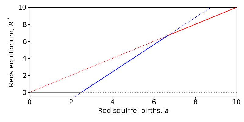
We can also plot a bifurcation diagram of the system. This is slightly complicated since we now have two variables and multiple parameters, but we can just focus on how one parameter impacts one variable. Here we see three different transcritical bifurcations at different points as we vary the red squirrel carrying capacity, [latex]a[/latex]:

• When [latex]a[/latex] is low, the Grey-only equilibrium (grey line with [latex]R=0[/latex]) is stable, the Red-only equilibrium (red line) is unstable and the coexistence equilibrium (blue) is negative (and unstable).
• When [latex]a[/latex] is intermediate, the coexistence equilibrium becomes positive and stable and the Grey-only equilibrium becomes unstable through a transcritical bifurcation. The Red-only equilibrium remains unstable.
• When [latex]a[/latex] is high, the coexistence equilibrium becomes unstable (and actually negative in [latex]G[/latex], though this plot does not show that) and the Red-only equilibrium becomes stable through a transcritical bifurcation. The Grey-only equilibrium remains unstable.

(There is a third transcritical bifurcation at 0 where the Red-only and Grey-only equilibria collide, but this makes no real difference to the dynamics since we assume [latex]a\gt 0[/latex]).

Chapter references

• The content in the Population ecology was influenced by the textbook, Mathematical Biology 1 by Murray.