A model for angiogenesis

In the last chapter we looked at a number of different ways we might model cancer dynamics, but did minimal analysis of these. In this chapter we will take a more in-depth look at one particular model where we consider the phsyical growth of a cancerous tumour (see chapter references).

We can model the size of a tumour by the number of cancer cells that make it up. These dynamics may actually be well represented by the logistic growth model we studied in the very first lecture (other forms, such as the Gompertz model, are often used instead, but the logistic model will do just fine). That is because tumours tend to slowly increase in size at first, then rapidly grow and finally saturate to a finite size due to resource limitations such as physical space and blood supply. Therefore, the density of cancer cells, [latex]c[/latex], in a tumour may be expected to obey the dynamics,

[latex]\begin{equation} \frac{dc}{dt}=r_0c\left(1-\frac{c}{K}\right) \end{equation}[/latex]

where [latex]r_0[/latex] is the basic growth rate and [latex]K[/latex] the carrying capacity.

An important feature of tumour growth, however, is that they can change their environment as they grow through angiogenic factors, such that they can both stimulate and inhibit their own growth. For example, as the tumour grows it can physically create more space to grow in to, as well as secrete chemicals that encourage blood vessels to grow. On the other hand as the tumour grows it may cause damage to the existing blood supply. By affecting their environment in this way, cancer cells are changing their own carrying capacity. Therefore, while we previously assumed a fixed carrying capacity, [latex]K[/latex], it now makes sense to treat this is a dynamic variable that may grow or shrink over time depending on these angiogenic processes. The model that is proposed for these dynamics is,

[latex]\begin{equation} \frac{dK}{dt}=\phi c - \theta Kc^{2/3}=c\left[\phi-\theta Kc^{-1/3}\right]. \end{equation}[/latex]

Cells stimulate the growth of blood vessels, and hence the carrying capacity, at individual-level rate [latex]\phi[/latex]. The inhibition rate, with parameter [latex]\theta[/latex], is rather more complicated and stems from the argument we made in the previous chapter about the volume of tumour, but applied to how tumour growth will damage local blood vessel networks.

Anaylsis

As usual, we will proceed by finding possible equilibria, classifying their stability and drawing phase portraits.

We already know from our previous work on the logistic model that,
[latex]\begin{equation} \frac{dc}{dt}=0\implies c=0 \textrm{ or } c=K. \end{equation}[/latex]

Substituting these values in to our second equation, we find that,

• if [latex]c=0[/latex], [latex]dK/dt[/latex]=0 for any [latex]K[/latex], and therefore there are a continuum of equilibria with no tumour but a positive carrying capacity.
• if [latex]c=K[/latex], [latex]dK/dt=0\implies c[\phi-\theta K^{2/3}]=0[/latex]. There are two different cases here. Firstly we could have [latex]c=K=0[/latex] or we could have [latex]c=K=(\phi/\theta)^{3/2}[/latex].

There are therefore two qualitatively different long-term solutions: either the tumour is absent (with the carrying capacity possibly at zero) or it is maintained.

We should now look at the stability of these equilibria. The Jacobian of the system can be found to be,

[latex]\begin{align*} J=&\left( \begin{array}{cc} r\left(1-2\frac{c}{K}\right) & \frac{rc^2}{K^2}\\ \phi-\frac{2}{3}\theta Kc^{-1/3} & \theta c^{2/3} \end{array} \right) \end{align*}[/latex]

The general case of [latex]c=0,K>0[/latex] is problematic because of the lower-left entry. Of course this was already a special case, being a line of equilibria. We will look at this again when we draw the phase portrait. Let us first focus on the special case of [latex]c=K=0[/latex]. In fact, we know that we have [latex]c=K[/latex] in all of these cases, which leads to a number of simplifications.

If we now look specifically at [latex]c=K=0[/latex] we find,

[latex]\begin{align*} J=&\left( \begin{array}{cc} -r & r\\ \phi & 0 \end{array} \right) \end{align*}[/latex]

Here we have [latex]tr=-r\lt0[/latex] and [latex]\det=-r\phi\lt0[/latex], meaning this equilibrium is always unstable.

For the full equilibrium, since we know that [latex]K=(\phi/\theta)^{3/2}[/latex], this simplifies to,

[latex]\begin{align*} J=&\left( \begin{array}{cc} -r & r\\ \frac{1}{3}\phi & -\phi \end{array} \right) \end{align*}[/latex]

We therefore have, [latex]tr=-r-\phi\lt0[/latex] and [latex]\det=2r\phi/3\gt0[/latex], meaning the equilibrium is always stable. Together, then, these results suggest that the tumour will always grow to a fixed size and, even with very low growth, low stimulation and high inhibition, the tumour will persist.

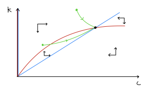
We can explore the behaviour further through plotting the phase portrait. As ever, we need to find the nullclines, determine the qualitative direction of flow, and sketch some trajectories.

Treatment

There are many ways to treat cancer, including through forms of chemotherapy and radiotherapy and an array of medication. Suppose we administered an anti-angiogenic drug, that reduces the carrying capacity of the tumour by limiting the blood supply. We will take a simple assumption that the drug causes a constant per-capita reduction in the carrying capacity (in reality it would be rather more complicated than this). We can model this by updating the second equation to include an additional mortality term, [latex]\mu[/latex],
[latex]\begin{equation} \frac{dK}{dt}=\phi c - \theta Kc^{2/3}-\mu K. \end{equation}[/latex]

After a few lines of working we can find that this changes the equilibrium values to be,
[latex]\begin{equation} c^*=K^*=\left(\frac{\phi-\mu}{\theta}\right)^{3/2}, \end{equation}[/latex]

or [latex]c^*=K^*=0[/latex].

Similarly the Jacobian changes to,
[latex]\begin{align*} J=&\left( \begin{array}{cc} -r & r\\ \phi-\frac{2}{3}\theta K^{2/3} & -\theta K^{2/3}-\mu \end{array} \right) \end{align*}[/latex]

and after substituting in the tumour equilibrium we find,
[latex]\begin{align*} J=&\left( \begin{array}{cc} -r & r\\ \frac{1}{3}\phi+\frac{2}{3}\mu & -\phi \end{array} \right) \end{align*}[/latex]

As before we have [latex]tr=-r-\phi\lt0[/latex], but we now have [latex]\det=r\frac{2}{3}[\phi-\mu][/latex]. Therefore when [latex]\mu[/latex] is high enough the equilibrium becomes unstable (and in fact it is quickly seen that this would be at the point when the equilibrium becomes negative, suggesting a transcritical bifurcation). We could also demonstrate this by re-plotting the phase portrait, which is left as an optional exercise.

Chapter references

• The model in this chapter is a much simplified version of that proposed by Hanhfeldt et al. (1999).