Auto-activation: a positive feedback

In the last chapter we introduced the general model for an auto-regulatory circuit for mRNA and protein dynamics,

[latex]\begin{align} \frac{dM}{dt} &= f(P) - \mu M\\ \frac{dP}{dt} &= kM - \nu P \end{align}[/latex]

and looked at the specific case of auto-repression where [latex]f'(P)\lt 0[/latex]. We will now look at the opposite form of autoregulatory genetic networks. If the protein product of a gene acts to increase the rate of transcription, we describe it as a transcriptional activator. The feedback circuit is described as auto-activation. In this case, [latex]f'(P)\geq0[/latex], i.e. [latex]f(P)[/latex] is an increasing function.

The equation for steady state values of [latex]P[/latex] is
[latex]\begin{equation} \frac{\mu\nu}{k}P=f(P) \end{equation}[/latex]

We know that [latex]f(P)[/latex] is increasing and bounded above, so what can we conclude about the number of equilibria? Depending on how weird and wonderful we make [latex]f(P)[/latex], there must be at least one, and there can be any odd number of equilibria. Realistically we’d expect one or three, since we probably wouldn’t choose a form for [latex]f(P)[/latex] that is too wild.

As before, the Jacobian is given by,

[latex]\begin{align*} J=&\left( \begin{array}{cc} -\mu & f'(P^*)\\ k & -\nu \end{array} \right), \end{align*}[/latex]

but now [latex]f'(P^*)\gt0[/latex]. The trace remains [latex]tr(J)=-\mu-\nu\lt0[/latex]. The determinant is again given by [latex]\det(J)=\mu\nu-k\phi[/latex], where [latex]\phi=f'(P^*)[/latex], but because [latex]\phi\lt0[/latex] it can be either positive or negative. We therefore have that,

• if [latex]\phi \lt \mu\nu/k[/latex], the equilibrium is stable,
• if [latex]\phi \gt \mu\nu/k[/latex], the equilibrium is a saddle.

We can go slightly further in the first case, by recalling that [latex]tr^2-4\det=(\mu-\nu)^2+4k\phi\gt0[/latex]. Therefore if the equilibrium is stable it will definitely be a node and not a spiral.

Using phase portraits

As it turns out, using this information, when we look at a phase portrait we can immediately spot whether an equilibrium is a stable node or a saddle. Consider the sketched nullclines in the figure below. This identifies three equilibria where the two nullclines cross in this case. The gradient of the blue line is [latex]\nu/k[/latex] and the gradient of the red line is [latex]f'(P)/\mu=\phi/\mu[/latex]. As we have just found, which of these two terms is greater – i.e. which is the steeper – controls the stability of each equilibrium. Therefore in the two cases where the blue line is steeper the equilibria are stable nodes, and in the case where the red line is steeper we have a saddle.

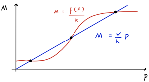
*Figure: example of nullclines for auto-repression model.*

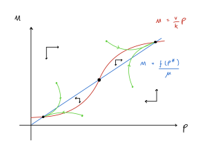
This system demonstrates bistability – there are two possible stable endpoints separated by an unstable saddle (we saw a similar case back when we looked at the competition model). This particular case is often called a bistable switch because the system can switch between high and low expression of the gene with small changes to the initial condiitons.

It is worth noting that we could equally have drawn the phase portrait with just one equilibrium. These must result in a single stable node (since the red nullcline must start from above and then cross below the blue nullcline), but can be at high or low gene expression depending on quite how we draw the two nullclines, as we will see below.

An example transcription function

You will have noticed we sketched our [latex]f(P)[/latex] nullclines in a sigmoidal shape. We saw something similar with the spruce budworm, predator-prey and within-host Covid-19 models. In this biological context they are often called Hill functions. The general formula for such a curve is,

[latex]\begin{equation} f(P)=\alpha+\beta\frac{P^n}{\theta^n+P^n}, \end{equation}[/latex]

where [latex]\alpha[/latex], [latex]\beta[/latex], [latex]\theta[/latex] and [latex]n[/latex] are all positive constants. The curve has the following key features:

• The curve starts at [latex]f(0)=\alpha[/latex],
• The gradient [latex]f'(P)\gt0[/latex],
• [latex]\theta[/latex] is the half-saturation constant, with [latex]f(\theta)=\alpha+\beta/2[/latex],
• [latex]n[/latex] controls how strong the sigmoidal shape is, and we usually assume [latex]n\geq2[/latex],
• As [latex]P\to\infty[/latex], [latex]f(P)\to\alpha+\beta[/latex].

Thinking more about the contribution of [latex]n[/latex], as this becomes larger, the transition from low to high transcription rates becomes more sudden and steep – we would describe this as increasing the sensitivity of the rate of transcription.

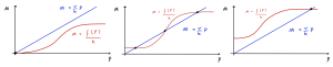
To see how we can use the parameters of the Hill function to switch gene expression from a low to high state, consider the effect of increasing the value of [latex]\alpha[/latex]. If we start with [latex]\alpha = 0[/latex] and [latex]\nu/k[/latex] large enough, then the only steady state is a stable node at [latex]P = 0[/latex] as in the first figure below. We say the system is monostable. In terms of the biology of the system, the gene is turned off.

If we now increase the value of [latex]\alpha[/latex], then provided the steepest part of the function has a gradient that is greater than [latex]\nu/k[/latex] , there is a range of values of [latex]\alpha[/latex] for which the system has three steady states. For this range of values of [latex]\alpha[/latex], the system is bistable, and has two possible stable steady state expression levels as shown in the second diagram.

If we increase [latex]\alpha[/latex] even further, then the system again has only one stable node steady state (monostability), but now it corresponds to a high level of expression of [latex]P[/latex], as in the final diagram. By increasing the value of [latex]\alpha[/latex], we have therefore switched the gene from a stable “off” state ([latex]P = 0[/latex]) to a stable “on” state ([latex]P[/latex] high).

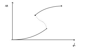
[latex]\alpha[/latex] can be considered as an external input to the system – a transcription rate that is independent of [latex]P[/latex]. We sometimes refer to [latex]\alpha[/latex] as a basal transcription rate. If the system is initially in the bistable region (with three steady states), but is in the low expression state (which is a stable node), then a transient increase in [latex]\alpha[/latex] can push the system into the monostable region, where only a high stable steady state exists. In other words, expression of the gene is turned on. If [latex]\alpha[/latex] is now returned to its original value, the system will remain in the steady state corresponding to a high level of expression. Thus, a transient externally-imposed impulse can stably switch the bistable system from a low to a high level of expression of an auto-activating gene. This is an example of hysteresis – the response of the system depends not only on its current input, but also on its history of past inputs. Whether or not such switching occurs depends on the speed and magnitude of the transient increase in [latex]\alpha[/latex].

Chapter references

• The content in the Gene networks section is based on the unpublished Mathematical Biology lecture notes developed by Nick Monk.