What is pharmacokinetics?

Pharmaco-kinetics is concerned with how drugs move around the body (see chapter references). In reality this is a highly complex process, as drugs are absorbed, distributed, metabolised and eliminated through various parts of the body. We will make various assumptions that mean we can simplify these processes. In particular we will assume the body is made up of just one or two compartments through which the drugs move. We will also simplify the processes by which drugs are administered. Our focus will be on how the concentration of a particular drug in the body changes over time. We are therefore continuing with ordinary differential equations as our go-to tool, but it is worth stressing that we have moved slightly away from what we might classically call biology (since nothing is actually living in these models) and more into medicine.

A single dose model

Let’s start with the simplest (yet realistic) model we can think of, and then we will gradually build more complexity in to it. Let us assume that:

• The body can be considered as a single compartment (effectively the bloodstream),
• There is rapid infusion of the drug in to the body as a single dose, called an intravenous bolus,
• Only one dose of the drug is administered,
• The drug is eliminated from the body at a rate proportional to the drug concentration.

Let [latex]C(t)[/latex] be the concentration of the drug in the bloodstream at time [latex]t[/latex]. If the rate of elimination of the drug is [latex]k[/latex], we can write,
[latex]\begin{equation} \frac{dC}{dt} =-kC, \end{equation}[/latex]

with some initial concentration [latex]C(0)=C_0>0[/latex]. Note that we only have a negative term on the right-hand side, indicating the concentration of the drug is always decreasing. This fits with our assumptions above intuitively, since we assume no additional drug is added after [latex]t=0[/latex], and so all that can happen to the drug is it is eliminated by the body.

This is a linear ordinary differential equation that is almost identical to the very first model that we met in this textbook (just with a minus sign). Using the same method of separation of variables we can find that,

[latex]\begin{equation} C(t)=C_0e^{-kt}. \end{equation}[/latex]

We thus predict exponential decay of the drug concentration.

Calculating [latex]k[/latex]

Suppose we wish to find out what the elimination rate is for a particular drug. All we need are two data-points for the concentration at known times. One of these could be the starting concentration ([latex]C_0[/latex] at [latex]t=0[/latex]), and suppose we take a measurement of the concentration, [latex]C_1[/latex] after [latex]t_1[/latex] hours. If we take logs of both sides of our solution we find,

[latex]\begin{align*} \ln(C_1)&=\ln(C_0)-kt_1\\ \implies k&=\frac{\ln(C_0)-\ln(C_1)}{t_1}. \end{align*}[/latex]
In fact, if we were to have multiple data points we simply need to know the gradient of the line of [latex]\ln(C(t))[/latex] vs [latex]t[/latex]. Given that [latex]k[/latex] is a rate it will have units [latex]t^{-1}[/latex]. Hourly elimination rates for real drugs tend to be in the range [latex]k\in[0.02,0.4][/latex].

A note on [latex]C_0[/latex]

We assumed above that we would know the initial concentration, [latex]C_0[/latex]. This seems obvious since we know what the dose was. However, we should note that dose and concentration are not the same thing. The dose is the actual amount of the drug administered, while the concentration is the relative amount of drug in the body as a proportion of the volume of the body. We can convert between the two by noting that [latex]C_0=dose/volume[/latex]. For slightly complex biological reasons, the effective volume is not necessairly as simple as just calculating a patient’s actual body (or blood) volume and varies from drug to drug. For simplicity, however, we will assume it is a fixed value for each drug in every patient.

Drug half-life

Given that we expect exponential decay of drug concentration over time, we cannot give a precise time when the concentration would be exactly zero. However, we can calculate a half-life for the drug based on its elimination rate. Assume we know the concentration is [latex]C_a[/latex] at some time point. Then to find the half-life we need to know the time until the concentration is [latex]C_a/2[/latex]. Using the logged solution from above, we have,

[latex]\begin{align*} \ln(C_a/2)&=\ln(C_a)-kt_{1/2}\\ \implies t_{1/2}&=\frac{\ln(C_a)-\ln(C_a/2)}{k}\\ \implies t_{1/2}&=\frac{\ln(2)}{k}. \end{align*}[/latex]

Click for solution

First, we can find the elimination rate, [latex]k[/latex], directly from the half-life, using,
[latex]\begin{align*} & t_{1/2}=\frac{\ln(2)}{k}\\ \implies & k=\frac{\ln(2)}{t_{1/2}}\\ \implies & k=0.231. \end{align*}[/latex]

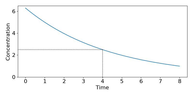
Next we will find out what the initial concentration must have been. We know that [latex]k=0.231[/latex] and that [latex]C(t=4)=2.5[/latex]. We can therefore use,
[latex]\begin{align*} &C(t)=C_0e^{-kt}\\ \implies &C_0=C(t)e^{kt}\\ \implies & C_0=2.5e^{0.231\times 4}=6.297 \text{mg/L}. \end{align*}[/latex]
The final step is to convert this to the actual dose by multiplying through by the volume to get dose[latex]=6.297\times30\approx 190[/latex]mg. A plot of the resulting dynamics is shown in the figure below.

Chapter references

• The content in the Pharmacokinetics section is based on the ebook, Basic Pharmacokinetics by Bourne.