regulatory feedback loops

In our first example, transcription of mRNA was due to some external signal or resource. However, many genes encode transcription factors that directly regulate the rate of transcription of the coding gene. This produces a small feedback circuit. Representing the concentrations of mRNA and protein by [latex]M(t)[/latex] and [latex]P(t)[/latex] again, we can now write,

[latex]\begin{align} \frac{dM}{dt} &= f(P) - \mu M\\ \frac{dP}{dt} &= kM - \nu P. \end{align}[/latex]

Now the concentration of protein directly influences the transcription of mRNA, producing this autoregulation feedback loop. The function [latex]f(P)[/latex] must be bounded above, since transcription must have some maximal rate. Furthermore [latex]f(P) \geq 0[/latex] (the production rate cannot be negative). Therefore [latex]f(P)[/latex] must be non-linear, which makes the system defined by the equations above difficult, if not impossible, to solve explicitly.

To gain insight into the possible dynamics of the system, we will use qualitative analysis based around the construction of the phase portraits and linear stability analysis.

Constructing the phase portrait

Nullclines

The nullclines of the system are given by,

[latex]\begin{align} &\frac{dM}{dt}=0 \implies M=f(P)/\mu\\ & \frac{dP}{dt}=0\implies M=\nu P/k. \end{align}[/latex]

These are both single lines/curves in the phase plane.

Equilibria

Putting the two nullcline equations equal to one another, we find a single equation for the possible equilibrium values of [latex]P[/latex]:

[latex]\begin{equation} \frac{\mu\nu}{k}P^*=f(P^*). \end{equation}[/latex]

In that case we can then find [latex]M^*=\nu P^*/k[/latex] to be the corresponding equilibrium for mRNA. We can therefore focus our attention on determining the nature of any solutions for [latex]P^*[/latex] for different forms of the function [latex]f(P)[/latex].

Linearisation

As in previous examples, we assess stability around an equilibrium by linearisation, through looking at the Jacobian. For this model our Jacobian is,

[latex]\begin{align*} J=&\left( \begin{array}{cc} -\mu & f'(P^*)\\ k & -\nu \end{array} \right). \end{align*}[/latex]

We then check the trace and determinant to assess stability:

• [latex]tr(J)=-\mu-\nu[/latex]
• [latex]\det(J)=\mu\nu-kf'(P^*)[/latex].

The trace is always negative, limiting stability to a stable spiral or node, or an unstable saddle. Which outcome we get depends on the determinant, which in turn depends on the gradient of our transcription function at the equilibrium, [latex]f'(P^*)[/latex]. We will now consider a few examples of what this function might look like.

Auto-repression: a negative feedback

If the protein product of a gene acts to reduce the rate of transcription, we describe it as a transcriptional repressor. The feedback circuit is described as auto-repression. In this case, [latex]f'(P)\leq 0[/latex], i.e. [latex]f(P)[/latex] is a decreasing function. For the most part we will not write down explicit forms for [latex]f(P)[/latex] but just rely on our qualitative knowledge about it.

Recall the equation for steady state values of [latex]P^*[/latex] is

[latex]\begin{equation} \frac{\mu\nu}{k}P^*=f(P^*). \end{equation}[/latex]

Since [latex]f(P)[/latex] is strictly decreasing, this has a unique solution for [latex]P^*\gt 0[/latex], as shown graphically below.

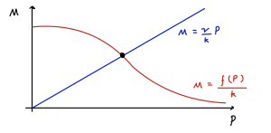
We therefore have one unique equilibrium. Let us call the value of [latex]f'(P^*)=\phi\lt 0[/latex] at the equilibrium. As such we can say that [latex]\det(J)=\mu\nu-k\phi[/latex] is positive, meaning the equilibrium is stable. Whether the equilibrium is a node or a spiral then depends on the value of,

[latex]\begin{align} tr^2-4\det &= (\mu+\nu)^2-4\nu\mu+4k\phi\\ &=(\mu-\nu)^2+4k\phi. \end{align}[/latex]

Firstly, we can see in the special case that [latex]\mu=\nu[/latex] (the two degradation rates are equal), we just have [latex]4k\phi\lt0[/latex], meaning we will have a stable spiral. More generally, there is a critical value,

[latex]\begin{equation} \phi_c=-\frac{(\mu-\nu)^2}{4k}, \end{equation}[/latex]

such that,

• if [latex]\phi\gt\phi_c[/latex] then we have a stable node,
• if [latex]\phi\lt\phi_c[/latex] then we have a stable spiral.

Recalling that [latex]\phi \lt 0[/latex], we see that [latex]f(P)[/latex] must be sufficiently steep at the equilibrium for it to be a spiral. The steepness of [latex]f(P)[/latex] (i.e. the modulus of the derivative of [latex]f(P)[/latex]) can be thought of as the sensitivity of the rate of transcription to changes in the protein concentration; high sensitivity means that a small change in the concentration of [latex]P[/latex] results in a large change in the rate of transcription. So sensitive regulation is more likely to lead to a stable spiral.

Sketching the phase portrait

We can now sketch the phase portrait for the case of an auto-repressive gene. Note that it is easiest to draw the phase portrait with the variable [latex]P[/latex] on the x-axis, and [latex]M[/latex] on the y-axis.

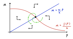
Note that if the equilibrium is a spiral, then trajectories spiral in a clockwise direction. The time courses [latex]M(t)[/latex] and [latex]P(t)[/latex] will be damped oscillations about their equilibrium values, with a peak in [latex]P[/latex] following a peak in [latex]M[/latex]. This makes sense biologically, since mRNA acts as a template for production of protein (by translation).

Chapter references

• The content in the Gene networks section is based on the unpublished Mathematical Biology lecture notes developed by Nick Monk.