Developing a 2-compartment model

So far we have assumed that as soon as the drug is administered it is immediately present in the bloodstream since it is administered intravenously. However, many drugs are administered in other ways, such as orally through tablets. In this case the drug will first reach the gastrointestinal (GI) tract where it dissolves and is gradually absorbed into the bloodstream. In this case we need to include two compartments in our model – one for the amount of the drug in the GI tract (which we might denote by [latex]X_G[/latex]), and one for the amount of the drug in the bloodstream ([latex]X_B[/latex]). Notice that I have used the word amounts here, as the concentration would have little meaning in the GI tract.

Let’s initially assume that there is a one-off dose of the drug. The amount of the drug in the GI tract cannot be increased, and simply reduces as it is absorbed in to the bloodstream. Hence, we can describe the dynamics of this first compartment as,

[latex]\begin{equation} \frac{dX_G}{dt}=-aX_G. \end{equation}[/latex]

For the second compartment we can assume all the drug that leaves the GI tract arrives in the bloodstream, and this then decays as before as the body uses up the drug. Hence, the second equation will be,

[latex]\begin{equation} \frac{dX_B}{dt}=V\frac{dC}{dt}=aX_G-kX_B=aX_G-kVC. \end{equation}[/latex]

Even before deriving the solutions to these equations, we can get a good qualitative picture of what might happen. The amount of drug in the GI tract will decay exponentially down towards zero. Initially, the drug concentration in the bloodstream will be very low, suggesting little being lost due to decay, but the amount being absorbed in to the bloodstream would be relatively high, meaning the concentration will initially increase. As time goes on, the amount of drug left in the GI tract will decrease until a point is reached that the absorption of new drug is less than the decay of existing drug, and the bloodstream concentration will reduce. Eventually we would expect the bloodstream concentration to also approach zero.

Let’s show this formally. We can solve this pair of equations in turn. The first is in a fairly simple form and just yields,

[latex]\begin{equation} X_G(t)=X_G(0)e^{-at}. \end{equation}[/latex]

We can then substitute this in to the second equation, to give,

[latex]\begin{equation} \frac{dX_B}{dt}=V\frac{dC}{dt}=aX_G(0)e^{-at}-kVC. \end{equation}[/latex]

This can be re-arranged in to the form,

[latex]\begin{equation} \frac{dC}{dt}+kC=\frac{aX_G(0)}{V}e^{-at}. \end{equation}[/latex]

Written in this form, we can see it is possible to solve this equation by use of an integrating factor.

The resulting concentration over time for some chosen parameter values is shown in the figure below. (Note, there is one special case we need to consider separately when [latex]a=k[/latex], which is left as an optional exercise).

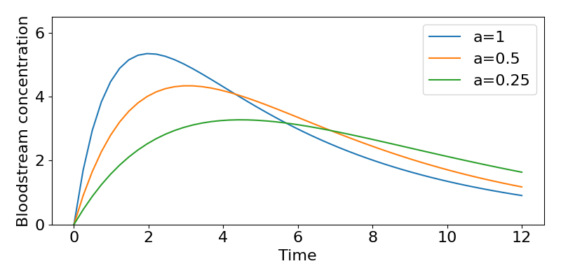
Consider our general solution, as shown in the figure. Notice that in theory the maximum possible concentration in the bloodstream would be [latex]X_G(0)/V[/latex] (which here would be 8mg/L) but due to the balance of absorption and decay this value is never reached (by some distance). What is the maximum concentration then? This peak is where the curve of the concentration becomes flat, which is by definition when [latex]dC/dt=0[/latex]. Hence we can find when it occurs by finding,

[latex]\begin{align} &\frac{aX_G(0)}{V}e^{-at}-kC=0\\ &\implies \frac{aX_G(0)}{V}\left[e^{-at}-\frac{k}{k-a}(e^{-at}-e^{-kt})\right]=0\\ &\implies ke^{kt}-ae^{-at}=0\\ &\implies \ln\left(\frac{k}{a}\right)=(k-a)t\\ &\implies t=\ln\left(\frac{k}{a}\right)\frac{1}{k-a}. \end{align}[/latex]

The faster the drug is absorbed into the bloodstream, the faster the concentration increases and the higher levels it reaches. However, this is at a cost of a faster loss of the drug as well. Plugging the values of [latex]a[/latex] in to the formula above, we find the peak concentration moves from 5.35mg/L at ~2 hours at the highest absorption rate, to 3.28mg/L at ~4.5 hours for the slowest rate of absorption.

Repeated oral doses

In this initial model we assumed a single oral dose. But, much like the intravenous bolus case previously, we will often give repeated doses of a drug. How will these concentrations change over time? We would probably expect to see curves rather like the previous case, with accumulation of the drug until some balance of dose and decay is achieved. In fact, we can see that for the amount of drug in the GI tract, [latex]X_G(t)[/latex], we will get exactly the same equations as for the intravenous bolus case. For the concentration of the drug in the bloodstream it is a bit more complicated, so we will think about things a little differently.

Let us assume that a dose is given every [latex]\tau[/latex] hours and let [latex]t[/latex] be the time since the last dose was given (meaning we always have [latex]0\lt t\lt\tau[/latex]). Sometime after the first dose, but before the second dose, the concentration of the drug, from above, is,

[latex]\begin{equation} C(t)=\frac{aX_G(0)}{V(k-a)}(e^{-at}-e^{-kt}). \end{equation}[/latex]

Now, sometime after the second dose the concentration will be made up of some contribution from the first dose plus a contribution from the second dose, such that,

[latex]\begin{equation} C(t)=C_1(t)+C_2(t)=\frac{aX_G(0)}{V(k-a)}(e^{-a(t+\tau)}-e^{-k(t+\tau)})+\frac{aX_G(0)}{V(k-a)}(e^{-at}-e^{-kt)}). \end{equation}[/latex]

Factoring out some terms and noting that [latex]e^{-a(t+\tau)}=e^{-at}e^{-a\tau}[/latex] gives,

[latex]\begin{equation} C(t)=\frac{aX_G(0)}{V(k-a)}(e^{-at}(1+e^{-a\tau})-e^{-kt}(1+e^{-k\tau})). \end{equation}[/latex]

Extrapolating we can see that after [latex]n[/latex] doses we will have,

[latex]\begin{equation} C(t)=\frac{aX_G(0)}{V(k-a)}(e^{-at}(1+e^{-a\tau}+...+e^{-(n-1)a\tau})-e^{-kt}(1+e^{-k\tau}+...+e^{-(n-1)k\tau})). \end{equation}[/latex]

We can see that there are two geometric series here, which will mean we can re-write this as,

[latex]\begin{equation} C(t)=\frac{aX_G(0)}{V(k-a)}\left(e^{-at}\left(\frac{1-e^{-na\tau}}{1-e^{-a\tau}}\right)-e^{-kt}\left(\frac{1-e^{-nk\tau}}{1-e^{-k\tau}}\right)\right). \end{equation}[/latex]

As before, we can find the maximum and minimum values by considering what happens as [latex]n\to\infty[/latex] and noting that the minimum concentration will always be as the new dose is taken, i.e. [latex]t=0[/latex]. Then,

[latex]\begin{equation} C_{\infty}(0)=\frac{aX_G(0)}{V(k-a)}\left(\left(\frac{1}{1-e^{-a\tau}}\right)-\left(\frac{1}{1-e^{-k\tau}}\right)\right). \end{equation}[/latex]

It may be that we can we assume that by this point there is negligible new drug being absorbed in to the body (in the case that the previous dose has virtually run out), and in that case we can take [latex]e^{-a\tau}\approx0[/latex] and therefore,

[latex]\begin{equation} C_{\infty}(0)\approx\frac{aX_G(0)}{V(k-a)}\left(-\frac{e^{-k\tau}}{1-e^{-k\tau}}\right). \end{equation}[/latex]

Calculating the maximum concentration is rather more tricky in this case as it is not simply at the start or end of the dosing interval. What we can do is to find the average concentration of the drug during one dose period ([latex]\tau[/latex]), defined as the area under the curve for one dose period at steady state,

[latex]\begin{equation} \bar{C}=\frac{1}{\tau}\int_0^{\tau}C_{ss}(t)dt. \end{equation}[/latex]

In fact we can make things easier by noting that this is equal to the whole area under the curve of the first dose on its own,

[latex]\begin{equation} \bar{C}=\frac{1}{\tau}\int_0^{\tau}C_{ss}(t)dt=\frac{1}{\tau}\int_0^{\infty}C_1(t)dt. \end{equation}[/latex]

Computing this integral we find,

[latex]\begin{align} \bar{C}&=\left(\frac{1}{\tau}\right)\left(\frac{aX_G(0)}{V(k-a)}\right)\int_0^{\infty}(e^{-at}-e^{-kt})dt\\ &=\left(\frac{1}{\tau}\right)\left(\frac{aX_G(0)}{V(k-a)}\right)\left[\frac{-e^{-at}}{a}+\frac{e^{-kt}}{k}\right]_0^{\infty}\\ &=\left(\frac{1}{\tau}\right)\left(\frac{aX_G(0)}{V(k-a)}\right)\left(\frac{-1}{a}+\frac{1}{k}\right)\\ &=\frac{X_G(0)}{Vk\tau}. \end{align}[/latex]

This average concentration can be useful in its own right. For instance, notice this means that a low dose at short intervals will give an equivalent average concentration as a high dose at long intervals. It can also be used to construct a crude approximation of the maximum concentration using [latex]C_+=\bar{C}+(\bar{C}-C_-)[/latex].

Example problems

Suppose an oral drug is prescribed for a patient with [latex]k=0.25, a=0.4, V=25[/latex] and a dose of 400mg is taken every 6 hours. Suppose that guidelines state the maximum safe concentration of the drug is 10mg/L and the minimum effective concentration is 5mg/L. Is this regime safe and effective?

Let us start by finding the minimum and maximum concentrations reached after repeated doses. If we do not make the assumption that absorption is negligible when the new dose is taken, we have,

[latex]\begin{equation} C_{-}=\frac{aX_G(0)}{V(k-a)}\left(\left(\frac{1}{1-e^{-a\tau}}\right)-\left(\frac{1}{1-e^{-k\tau}}\right)\right). \end{equation}[/latex]

Substituting in the values we have this gives, [latex]C_-=8.0[/latex]mg/L. We can also find the average concentration at steady-state using,

[latex]\begin{equation} \bar{C}=\frac{X_G(0)}{Vk\tau}, \end{equation}[/latex]

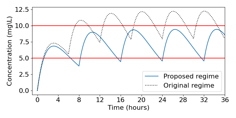
which gives [latex]\bar{C}=10.67[/latex]mg/L and we can use this to estimate the maximum concentration as [latex]C_+=13.3[/latex]mg/L (the plot below reveals this is in fact an over-estimate). Comparing these values to the guidelines, it is clear that this regime would reach doses which are much too high. Let us therefore devise a new regime.

Firstly, we can find that [latex]\bar{C}=(C_+-C_-)/2=7.5[/latex]mg/L. Substituting in to the formula for [latex]\bar{C}[/latex] we can say,

[latex]\begin{equation} X_G(0)=46.9\tau. \end{equation}[/latex]

We can substitute this back in to the equation for the minimum concentration, however there is no easy way to solve this analytically. What we can do is to solve it numerically. To do this we could plot the right-hand side for varying [latex]\tau[/latex] and look for where it equals 5. Doing this we find that the optimum timing is [latex]\tau=7.2[/latex] hours, which means [latex]X_G(0)=332[/latex]mg. We might well look to take a more realistic value of [latex]\tau=8[/latex] hours, giving [latex]X_G(0)=375[/latex]mg. The resulting dynamics for both the original and proposed regimes are shown below, revealing that our proposed regime indeed does a much better job of fitting the guidelines.

Chapter references

• The content in the Pharmacokinetics section is based on the ebook, Basic Pharmacokinetics by Bourne.