
4 Epidemics in human populations
the Susceptible-Infected-Recovered model
At the time of writing, it seems reasonable to say that mathematical modelling of disease spread has never been as topical or well-known amongst the general public. Many modellers and scientists have been contributing to our understanding of the Covid-19 pandemic, from research being conducted and published, to directly advising government policy, to public engagement and information. In the next few chapters we will cover the fundamentals of the mathematical models that are the basis of most of this modelling work. The models that have been used to advise governments are of course rather more detailed than those you will see here (and we’ll discuss some extensions as we go along), but there is a common engine behind them all.
Our first few models focussed on the dynamics of ecological populations. As part of this we have assumed that every individual within each population is identical. Such a generalisation has the benefit of reducing our model to a low number of variables. But often certain individuals within a population are fundamentally distinct from one another. In this case, we might want to divide our population up in to different compartments. The choice of how to divide our population is often dictated by the biological question we are seeking to address. For example we may wish to have an age-structured model, with adults and juveniles, or perhaps individuals with different roles in a population such as foragers or workers.
For the next few chapters we will focus on epidemic models, where we will need to use such a compartment model. Broadly, we will think about disease dynamics within populations of humans, animals or plants that act as hosts for diseases such as viruses or bacteria, often termed parasites or pathogens. We will initially assume we are interested in infectious diseases of human populations, and this will guide our model design. When thinking about the spread of disease through a population, while we might have some interest in the total population at any time, it is more likely that we want to know about individuals’ infection status – are they currently infected, for example. This will be the basis of our compartment model. Let’s draw a schematic diagram to picture this process:

Before a disease emerges, all individuals in the population are susceptible. Once exposed to the disease, individuals may then become infected (and also infectious). Finally, individuals will eventually fight off the disease to become recovered and immune.
This is the ‘SIR’ model (i.e. Susceptible, Infected, Recovered), and has been central to our understanding of disease dynamics in human populations since it was first proposed in the 1920s. Disease is transmitted by ‘direct contact’ between infected and susceptible hosts and is a ‘mass action’ process, meaning we do not take any account of contact networks and the risk of infection is proportional to the total density of infection in the population. When hosts have recovered, they gain immunity and cannot be infected again (this is a key aspect of vertebrate – and especially human – immune systems, but is not necessarily true of invertebrates, plants, etc. We will consider models more appropriate for such populations later). [latex]\beta[/latex] controls the rate at which contacts between [latex]S[/latex] and [latex]I[/latex] hosts cause infection, and [latex]\gamma[/latex] is the rate of recovery. A small personal pet peeve – [latex]\beta[/latex] itself is not a rate; it has the wrong units. In this initial example we have not included any birth or death processes, as we assume that infection happens at a much faster timescale than demography. By considering our schematic diagram above we can write down the dynamics of our system as a set of ODEs:
[latex]\begin{align} &\frac{dS}{dt} = -\beta SI\\ &\frac{dI}{dt} = \beta SI - \gamma I\\ &\frac{dR}{dt} = \gamma I \end{align}[/latex]
with the total population, [latex]N=S+I+R[/latex]. There are some useful definitions it is worth making at this point:
- [latex]\beta I[/latex] is often called the force of infection (this really is the rate of infection);
- [latex]I/N[/latex] gives the prevalence of infection;
- [latex]1/\gamma[/latex] is the infectious period.
One thing to spot is that [latex]dN/dt = dS/dt+dI/dt+dR/dt=0[/latex]. This means that the total population stays at a constant size (if we stop and think for a moment you might realise that this was built into our model all along since we have no births, deaths or migration). We can argue that this is a reasonable assumption for a short epidemic outbreak in long-lived human populations. An advantage of this assumption is that we can eliminate one variable, with [latex]R=N-(S+I)[/latex] and ignore the [latex]dR/dt[/latex] equation. This is because since the total population is always [latex]N[/latex], once we’ve worked out the densities of [latex]S[/latex] and [latex]I[/latex] we can immediately calculate the remaining density who must be [latex]R[/latex]. We therefore can write down the simplified model as,
[latex]\begin{align} &\frac{dS}{dt} = -\beta SI \\ &\frac{dI}{dt} = \beta SI - \gamma I \end{align}[/latex]
Analysis
Once again we have what looks to be a fairly simple set of ODEs (two variables and two parameters), but there exists no explicit solution due to the non-linear term [latex]\beta SI[/latex]. However, we can again explore the qualitative behaviour of the model by identifying equilibria of the system, assessing their stability and sketching phase portraits.
First let’s look for equilibria. The only way both ODEs can be 0 simultaneously is if [latex]I=0[/latex] (and [latex]S[/latex] may take any value less than [latex]N[/latex]). This means we have a line of non-isolated equilibria where there are no infected individuals in the population. This is another special case for stability as we would find that one of the eigenvalues is always zero. We will consider quite what is going on here when we sketch the phase portraits.
Before we do that, let us think a bit more about the general behaviour of the model. It is often the case with emerging diseases that they will eventually burn out, as we seem to be predicting here. But it is still important for us to know whether there can be an epidemic, when an initially small amount of infection causes a large outbreak of disease in the population (even if it eventually tends to zero). Taking this definition, for an epidemic to occur we need to have [latex]dI/dt \gt 0[/latex] initially. Before an outbreak, the initial densities are [latex]S(0)\approx N,I(0)\approx0[/latex]. This gives,
[latex]\begin{equation} \frac{dI}{dt}\approx(\beta N-\gamma)I \end{equation}[/latex]
This gives us a condition for an epidemic:
- [latex]\beta N-\gamma\lt 0[/latex] [latex]\implies[/latex] disease dies out.
- [latex]\beta N-\gamma\gt 0[/latex] [latex]\implies[/latex] epidemic.
So even though the ultimate dynamic is for the disease to die out, we can have an epidemic if the initial amount of infection outstrips the rate of recovery.
Let’s now draw phase portraits of our SIR model for the two scenarios we have found above. To find the nullclines we take,
[latex]\begin{align} &\frac{dS}{dt} = 0 \implies S=0, I=0\\ &\frac{dI}{dt} =0 \implies S=\frac{\gamma}{\beta},I=0 \end{align}[/latex]
Exercises
Click for solution
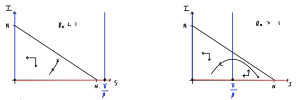
The two plots are sketched below. The first thing to notice is that in both plots only a triangular region bounded by the axes and [latex]I=N-S[/latex] is feasible. That is because if we took other positive values of [latex]S[/latex] and [latex]I[/latex] we would have [latex]S+I\gt N[/latex] which would not be possible given our fixed population size. In both diagrams we can quickly see that [latex]S[/latex] should be decreasing everywhere (since [latex]dS/dt\lt0[/latex]). In the first diagram we only have one region to worry about the qualitative direction of flow of [latex]I[/latex], since the vertical nullcline at [latex]S=\gamma/\beta[/latex] is outside the feasible region. In the second diagram we have two regions, towards the right [latex]I[/latex] increases and towards the left it decreases.
Remember where two (different) nullclines intersect is necessarily an equilibrium. Since both ODEs give a nullcline at [latex]I=0[/latex] we reinforce the fact that we have a continuum of equilibria along the line [latex]I=0[/latex]. Using our equations we can then find out in what regions [latex]S[/latex] and [latex]I[/latex] will be increasing or decreasing. Again, note it doesn’t matter that we can’t say precisely the direction of a trajectory anywhere on our plot; knowing the qualitative direction of travel gives us all the information that we need.
In the first case, the vertical nullcline at [latex]S=\gamma/\beta[/latex] does not appear in the feasible region, so actually has no impact on the dynamics. In fact we will always just drop down towards [latex]I=0[/latex] and the disease dying out. In the second case, the phase portrait is divided into two regions. If we start in a region to the right of the nullcline, the infected density initially increases – we have an epidemic – before crossing the vertical nullcline and approaching [latex]I=0[/latex] again. Therefore the equilibria where [latex]S\lt\gamma/\beta[/latex] appear to be locally stable (which it turns out is equivalent to the second eigenvalue being negative).
The divide between these two cases is whether [latex]N\gt \gamma/\beta[/latex] or not. We can rearrange this to the condition [latex]\beta N/\gamma\gt 1[/latex]. This ration is known as [latex]R_0[/latex], so we have the if [latex]R_0\gt1[/latex] we get an epidemic but if [latex]R_0\lt1[/latex] the disease dies out.
The basic reproductive ratio, [latex]R_0[/latex]
There is a very strong chance you have heard the terms [latex]R_t[/latex] or [latex]R_0[/latex] in discussions about the speed of spread of Covid-19. We define [latex]R_0=\beta N/\gamma[/latex] as the basic reproductive ratio of the disease: ‘The average number of secondary infections caused by one infected host in an otherwise disease-free population.’ Note that [latex]\beta N[/latex] gives the total infections caused in a disease-free population, and [latex]1/\gamma[/latex] is the infectious period. So [latex]R_0[/latex] gives the number of infections caused by an individual in the time that it’s infected near the start of an epidemic. The more general term, [latex]R_t=\beta S/\gamma[/latex] gives the number of new infections per case later in the epidemic when many individuals have already been infected and/or recovered. Because [latex]R_0[/latex] has this rather intuititve definition, it is a value that can often be estimated or measured. A number of estimates for [latex]R_0[/latex] of different diseases are given below. Remember, this figure tells you (roughly) how many new people an infected person will infect.
| Disease | [latex]R_0[/latex] |
|---|---|
| Flu | 1-3 |
| Covid-19 | 2-5 |
| SARS | 2-5 |
| HIV | 2-5 |
| Smallpox | 5-7 |
| TB | 8-10 |
| Measles | 12-18 |
Estimates of [latex]R_0[/latex] for some important human diseases.
The epidemic curve
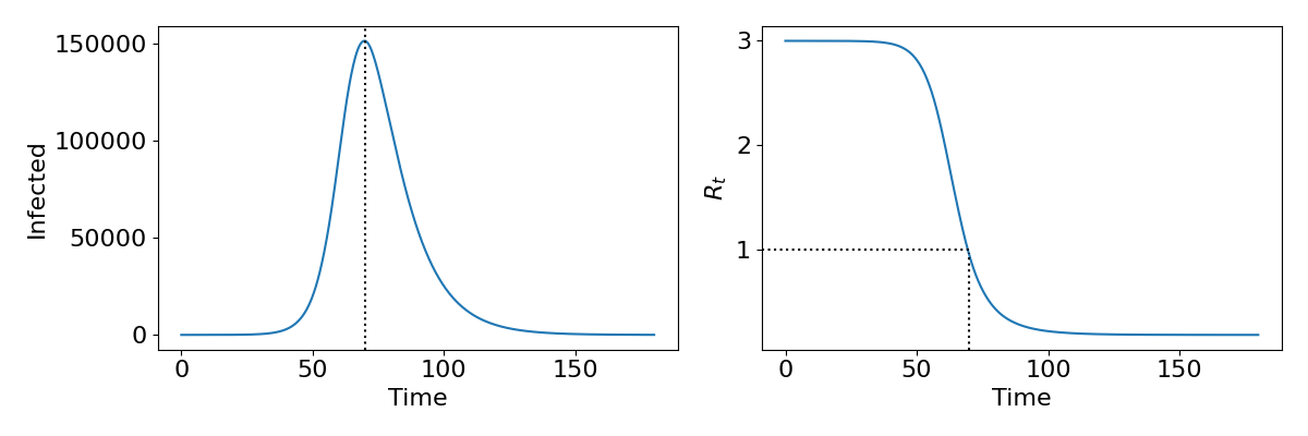
The phase portraits demonstrate again that an epidemic should always burn out and the population return to being disease-free. Interestingly the phase portraits also suggest that not all of the population will get infected during an epidemic, since we usually do not end with [latex]S=0[/latex] and [latex]I=0[/latex] (which would mean [latex]R=N[/latex]). As we have already said, due to the non-linearity of the system we are unable to find an exact solution and therefore cannot say precisely what the dynamics should look like. However, it is useful to understand what the epidemic curve – the number of people infected over time – looks like. With some approximations it is possible to express this as a mathematical formula, but we shall just look at some numerical output as shown in the left-hand side of the figure. This gives a characteristic bell-shaped curve. This is in fact the sort of curve we see from data from many real-world epidemics, suggesting that even our simple model is capturing something fundamental about disease spread. In the right-hand side we show how the reproductive ratio [latex]R_t[/latex] changes during the epidemic. Notice that the peak of the epidemic is precisely at [latex]R_t=1[/latex]. This will be important later when we discuss the idea of herd immunity.
Explore the model
Use the Python code below to explore the SIR model. In particular, this code will take an alternative approach by presenting the output from a stochastic simulation algorithm.
When using differential equations – as we are focussing on in this course – the models are deterministic meaning for the same parameter values and initial conditions you get the exact same dynamcis every time. In a stochastic model we account for variation in the parameters – for example in the ODE model a recovery rate of [latex]\gamma=1/7[/latex] is effectively interpreted as saying everyone recovers after exactly 7 days, whereas in a stochastic model we instead assume the recovery rate of each individual is drawn from a distribution where 1/7 is the mean. This means we get slightly different time-courses every time we run the model.
The code below will run 20 stochastic simulations as well as the deterministic equivalent. How good an approximation is the deterministic model to the stochastic one? Can you think of ways you might communicate the variation in the time-courses to policy makers or the public? Try changing the value of [latex]R_0[/latex] to see how the behaviour and differences change.
Click for code
# Import the necessary librariesimport numpy as npimport matplotlib.pyplot as pltfrom scipy.integrate import solve_ivp# Options to make the plot the right sizeplt.rcParams['figure.figsize'] = [8, 4]plt.rcParams.update({'font.size': 16})#Parameter valuesN=1000 GAMMA=1/14R0=2.5BETA=R0*GAMMA/NREPS=20 # Number of times to run the stochastic model
I0=2 # Starting number of infected individuals
# STOHASTIC MODEL CODE# Function to count numbers in each compartmentdef count_type(type): current_type=0; for i in range(0,N): for j in range(0,N): if grid[i,j]==type: current_type=current_type+1 return current_type# Function to check the current scaledef findscale(): S=susceptibles[-1] I=infecteds[-1] #Set relative parameter values scale=GAMMA*I+BETA*S*I return scale# Main functionfor reps in range(0,REPS): # Set initial conditions tsteps=[0] infecteds=[I0] susceptibles=[N-I0] current_t=0 # Main run of stochastic model while current_t<180: # Find time step scale=findscale() dt = -np.log(np.random.rand()) / scale current_t=tsteps[-1] tsteps.append(dt+current_t) #Find which event happens if np.random.rand()<GAMMA*infecteds[-1]/scale: #Event is recovery infecteds.append(infecteds[-1]-1) susceptibles.append(susceptibles[-1]) else: #Event is transmission infecteds.append(infecteds[-1]+1) susceptibles.append(susceptibles[-1]-1) if infecteds[-1]==0: break # Plot latest run if reps==0: plt.plot(tsteps,infecteds,':',color='blue',alpha=0.5,label='Stochastic model') else: plt.plot(tsteps,infecteds,':',color='blue',alpha=0.5)# ODE MODEL# Function to run model called 'disease'def disease(t,x): sdot=-BETA*x[0]*x[1] idot=BETA*x[0]*x[1]-GAMMA*x[1] return sdot, idot # Time points to use in ODE modelts=np.linspace(0,180,2000)# Run ODE model using 'solve_ivp'xx1=solve_ivp(disease,[ts[0],ts[-1]],[N-I0,I0],t_eval=ts) # Plotting commandsplt.plot(ts,(xx1.y[1]),'k',label='ODE model') plt.legend()plt.xlabel('Time')plt.ylabel ('No. Infected')plt.xlim(0,180)Key Takeaways
- We can model diseases using a compartment framework called the SIR model.
- An epidemic will occur when [latex]dI/dt[/latex] is initially positive, but in the simplest model will always reach an equilibrium where [latex]I=0[/latex].
- We can measure how quickly a disease initially spreads using [latex]R_0[/latex], and this tells us with there will be an epidemic or not.
Chapter references
- The content in the Infectious diseases section was influenced by the textbooks, Mathematical Biology 1 by Murray and Modelling Infectious Diseases in Humans and Animals by Keeling & Rohani.
