A simple predator-prey model

In the previous chapter we studied a first example of interacting populations with two species who compete with one another largely indirectly. Another common interaction that is much more direct is predation. Many species rely on others as a primary food source: foxes and rabbits; lions and zebras; ladybirds and aphids to name just a few. Such predator-prey interactions will have a similar structure to the competition models we considered last time, except that now one species (the predator) benefits from the interaction.

We will not start with the logistic model this time, but instead think of the simplest possible way we can model the dynamics of a prey with density [latex]N[/latex] and predator with density [latex]P[/latex],

[latex]\begin{align} \frac{dN}{dt} & =N(a-b P)\\ \frac{dP}{dt} &=P(-c+dN). \end{align}[/latex]

The prey has a birth rate [latex]a[/latex], no intraspecific competition and its death rate is only due to predation. This death from predation depends on the predator density (with parameter [latex]b[/latex]) with more predators leading to higher prey death and no saturation of predation at higher densities. In contrast, the predator’s birth rate depends on its ability to predate, and so depends on the prey density (with parameter [latex]d[/latex]). It has a simple death rate however at per-capita rate, [latex]c[/latex]. We might expect the parameters [latex]b[/latex] and [latex]d[/latex] to be linked, since one controls the amount of predation and the other the ability to reproduce which itself depends on predation. In some models you will see the predator birth term written as something like [latex]\theta bPN[/latex], where [latex]\theta[/latex] is the ‘conversion’ of energy from feeding into new births.

We have already identified a few simplifications we have made here even compared to our first few models – no intraspecific competition and continually increasing predation. A good approach to modelling is always to start with the simplest reasonable model and then build increasing complexity as needed. This is also the ‘classic’ predator-prey model you will see elsewhere, so it seems sensible to cover it here.

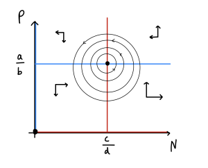
Let’s begin our analysis by finding the equilibria of the model. There is an extinction equilibrium at [latex](N,P)=(0,0)[/latex], and a coexistence equilibrium at [latex](N,P)=(c/d,a/b)[/latex]. The stability of these steady states is calculated, as before, by finding the Jacobian of the system.

We can quickly see that the extinction equilibrium, [latex](N,P)=(0,0)[/latex], is always unstable (since [latex]a>0[/latex]). What about the coexistence equilibrium? This evaluates to:

[latex]\begin{align} J=&\left( \begin{array}{cc} 0 & -bc/d\\ ad/b & 0 \end{array} \right), \end{align}[/latex]

Here, [latex]tr=0[/latex] and [latex]\det=ac>0[/latex]. These conditions mean that the eigenvalues at this equilibrium have zero Real part and are purely Imaginary. The behaviour near the steady state is therefore ‘centres’, a family of neutrally-stable closed orbits around the equilibrium. We therefore predict that these two populations will constantly cycle. With low predation the prey density increases; this produces more food for predators, and so the predator numbers begin to rise; this in turn starts to push the prey numbers back down; finally, with their food supplies falling, the predator numbers also drop down. A phase portrait of these dynamics would look like this,

Such a result initially seems appealing- this fluctuating behaviour makes intuitive sense and seems in line with some data from real systems. However, being centres these cycles are not structurally stable. The fact that if we make a change to the initial values we end up on a slightly different cycle is definitely mathematically unsatisfying and also questionable biologically. Let us see if we can update our model and get a stronger result.

A more realistic model

From our previous models we might already think of two additions to make the model more realistic. One is that we ignored intraspecific competition (i.e. no carrying capacity), meaning prey in particular could grow to infinite levels. Another is that we assumed predation was linearly dependent on prey density, whereas in the spruce budworm model we argued it should be saturating. Including these assumptions modifies the model to,

[latex]\begin{align} \frac{dN}{dt} &=N\left(a-\frac{b P}{N+A}-\alpha N\right)\\ \frac{dP}{dt} &=P\left(-c+\frac{dN}{N+A}\right). \end{align}[/latex]

Again we can start by looking for equilibria. We can see we still have the equilibrium at [latex](0,0)[/latex], and some coexistence equilibrium [latex](N^*,P^*)[/latex]. There is now also a new ‘prey-only’ equilibrium at [latex](N,P)=(a/\alpha,0)[/latex] . To assess stability we will need to also update our Jacobian, which is now,

[latex]\begin{align} J=&\left( \begin{array}{cc} a-\frac{bP}{N+A}-2\alpha N+\frac{bPN}{(N+A)^2} & \frac{-bN}{N+A}\\ \frac{dAP}{(N+A)^2} & -c+\frac{dN}{N+A} \end{array} \right), \end{align}[/latex]

The extinction equilibrium will remain a saddle always, which can be seen by using the Jacobian or simply considering the dynamics of the two species near that point. Let us look in more detail at the two other equilibria.

Prey-only equilibrium

In this case the Jacobian reduces to,

[latex]\begin{align} J=&\left( \begin{array}{cc} -\alpha N & \frac{-bN}{N+A}\\ 0 & -c+\frac{dN}{N+A} \end{array} \right), \end{align}[/latex]

Noting that we have a 0 in the bottom-left, we can read off our eigenvalues as [latex]\lambda_1=-\alpha N^*\lt0[/latex] and [latex]\lambda_2=-c+dN^*/(N^*+A)[/latex]. Therefore stability depends on [latex]\lambda_2[/latex], which is actually the growth rate of predators near this equilibrium (i.e. with near-zero predator densities). If the growth rate is negative the prey-only equilibrium is stable, but if it is positive the prey-only equilibrium is a saddle, which seems like what we would expect.

Coexistence equilibrium

As in the example with competition, we have not yet written out the densities for the prey and predators at the coexistence equilibrium, but we can still assess its stability by using the fact we are at the equilibrium. This means we know that [latex]a-b P/(N+A)-\alpha N=0[/latex] and that [latex]-c+dN/(N+A)=0[/latex]. Substituting these into the Jacobian leads us to,

[latex]\begin{align} J=&\left( \begin{array}{cc} -\alpha N+\frac{bPN}{(N+A)^2} & \frac{-bN}{N+A}\\ \frac{dAP}{(N+A)^2} & 0 \end{array} \right), \end{align}[/latex]

In this case we need to use the trace and determinant to assess stability. We can find that the determinant is given by, [latex]\det=bdAN^*P^*/(N^*+A)^3\gt0[/latex], and the trace by, [latex]tr=-\alpha N^*+bN^*P^*/(N+A)^2[/latex]. Stability therefore depends on whether the trace is positive or negative, which we can see depends on the balance of intraspecific competition in the prey and predation: if competition is high relative to predation, we will have a negative trace and the equilibrium is stable; if predation is high relative to competition, we will have a positive trace and the equilibrium is unstable.

Notice that if we vary one parameter, [latex]\alpha[/latex], say, we could move the system from being a stable spiral to being an unstable spiral, since we move from a negative to a positive trace. This is a change in stability, and therefore a bifurcation, but one that we have not yet seen in practice and which cannot occur in one-dimensional systems.

Hopf bifurcation

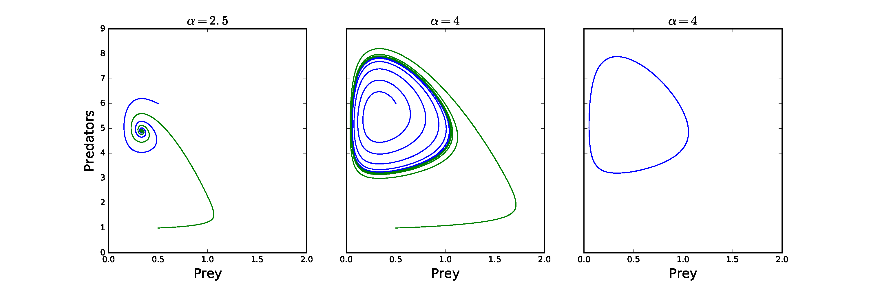
This transition is called a Hopf bifurcation. In this case changing a parameter turns a stable spiral in to an unstable spiral (or vice versa). This is a particularly important behaviour, because as we initially move into the unstable spiral region, a unique, stable closed orbit emerges from the equilibrium (see the background review chapter). This results in the population cycling/oscillating, and the orbit is called a limit cycle. It is not very easy to draw a bifurcation diagram in this case, but we can see the process by looking at the phase portraits as we vary a parameter.

The example in the figure below comes from our predator-prey model we have just examined. Here we see we initially have a stable spiral into the coexistence equilibrium, but that as we increase [latex]\alpha[/latex] the equilibrium loses stability and starts to spiral away. However, this outward trajectory does not continue to spiral out but tends towards a closed orbit (which can be seen clearly in the right-hand figure where I only plotted later time-points). An initial condition from further away starts to spiral in but also approaches this closed orbit. This is a much stronger result for population cycles than the centres we saw in the simple model. Hopf bifurcations have important consequences as populations which are fluctuating may be much harder to measure or control.

Chapter references

• The content in the Population ecology section was influenced by the textbook, Mathematical Biology 1 by Murray.