A quick guide to cells and genetic networks

In the next few chapters, we will look at models for the regulation of gene expression in cells, and how simple feedback loops underlie some of the basic dynamics that cells exhibit: regulation, switching, and oscillation.

From experience, undergraduate mathematics students are often familiar enough with ideas in ecology or epidemiology to follow the biological aspects of our models well enough without too much extra detail. However, many have little knowledge of cell dynamics and genetics. So, before we start introducing the models themselves we will have a short primer of what it is we are trying to model (and I hope any biologists will forgive me my simplifications and mistakes!)

All living things are made of cells – self-contained structures bounded by a cell membrane (and sometimes also a cell wall). Many organisms exist predominantly as single cells (e.g. bacteria, amoebae), while others exist as patterned collections of cells (e.g. animals, most plants). While different cells possess and maintain a well-defined identity, they are far from static structures, and depend on balanced dynamical processes. Mathematical modelling plays an important role in understanding these dynamical processes and how they are regulated in cells.

Unicellular organisms encounter variable environments, and therefore need to be able to adapt their behaviour. For example, a bacterium living in your gut will have to adapt its metabolism to whatever food you present it with, an example where a cell must switch between different behaviours. Multicellular organisms often develop from a single cell through sequential rounds of cell division. However, the cells in multicellular organisms do not remain identical to each other, but take on stable and well-defined characteristics, so we can talk about skin cells, liver cells, muscle cells, blood cells, etc. in a meaningful way. This adoption of distinct well-defined characters is called differentiation, and again requires cells to be able to switch their behaviour.

How do cells manage to change or switch their state in a coherent way? They use a combination of information from their environment and internal mechanisms. Central to the internal mechanisms are what we call gene regulatory networks. Almost all cells contain large structures centred on DNA (deoxyribonucleic acid), basically a set of long, linear sequences of letters (A, C, G and T). This sequence is highly stable, is accurately copied during cell division, and is identical in all cells of a multicellular organism. The full DNA sequence in a cell is referred to as the genome.

How is the genome involved in the regulation of the state of a cell, either stably maintaining it or switching it? A key concept is that of the gene, and the basic unit of dynamics that we will concern ourselves with here is the expression of a gene. For our purposes, a gene is a defined subset of the DNA sequence that can code for (can be copied, or transcribed to) an mRNA molecule. In turn the mRNA produced from the gene codes for (can be translated into) a particular protein molecule. We will refer to the regulated production and degradation of the mRNA and protein corresponding to a gene as the expression of that gene. The amount of the gene itself does not change, and so the dependent variables of our models will be the concentrations of mRNA and protein in a cell.

Initially, we will consider the regulated expression of a single gene. Later, we will consider how genes can interact by regulating each others’ expression. We will again focus exclusively on differential equation models, in which the concentrations/amounts of mRNA and protein are represented by continuous variables. These are essentially population models, just like the ones in the textbook so far.

A first model

In these models, we will consider the dynamics of gene expression in two scenarios:

1. The expression of the gene is regulated by some external transcription factor (whose concentration may or may not be a function of time).
2. The expression of the gene is regulated by its own protein product (which is therefore a transcription factor).

The models have two variables: [latex]M(t)[/latex], the concentration of mRNA, and [latex]P(t)[/latex] , the concentration of protein. The dynamics of [latex]M(t)[/latex] and [latex]P(t)[/latex] are regulated by production and degradation. These are similar to what we would formerly have called births and deaths, but those terms don’t really make biological sense to use here. In this context, the molecular processes underlying the production of mRNA and protein are called transcription and translation, respectively.

We will make the following assumptions:

1. The rates of mRNA and protein degradation are proportional to their concentration (i.e. degradation is linear).
2. The rate of translation is proportional to the mRNA concentration (i.e. translation is linear).

Then the general form of the models, written as a pair of ordinary differential equations, is

[latex]\begin{align} \frac{dM}{dt} &= R(t) - \mu M\\ \frac{dP}{dt} &= kM - \nu P. \end{align}[/latex]

where [latex]\mu[/latex] is the degradation rate of mRNA, [latex]\nu[/latex] is the degradation rate of protein, [latex]k[/latex] is the translation rate, and [latex]R(t)[/latex] is the transcription rate. Note that for the model to make sense biologically, [latex]\mu[/latex], [latex]\nu[/latex] and [latex]k[/latex] must be positive constants, and [latex]R(t) \geq 0[/latex]. Note also that if [latex]R(t)[/latex] is not constant, then the model will not go to an equilibrium.

Constant transcription

Let’s get as far as we can analysing this model and then think about this tricky translation term [latex]R(t)[/latex]. Starting with the dynamics of mRNA expression, we see that it is linear in [latex]M[/latex] and independent of [latex]P[/latex], so we can solve it in isolation by using an integrating factor. We have
[latex]\begin{equation} \frac{dM}{dt} +\mu M = R(t). \end{equation}[/latex]

Note we don’t have a fully explicit solution here; it is clear that [latex]R(t)[/latex] is going to be very important for how the time course plays out. Let us initially assume that [latex]R(t)=r[/latex], that is, we have constant transcription. As such we can simplify the equation to,

[latex]\begin{equation} M(t) = re^{-\mu t}\int e^{\mu t}dt. \end{equation}[/latex]

This gives us a function we can integrate, so our solution becomes,

[latex]\begin{align} M(t) &= \frac{r}{\mu}e^{-\mu t}\left[e^{\mu t}+C\right],\\ &= \frac{r}{\mu}\left[1+Ce^{-\mu t}\right], \end{align}[/latex]

where [latex]C[/latex] is a constant of integration. Now let us assume we know the initial concentration of mRNA at time [latex]t=0[/latex] is [latex]M_0[/latex]. We can use this to find our constant of integration as,

[latex]\begin{equation} C=\frac{M_0\mu}{r}-1. \end{equation}[/latex]

Substituting back in allows us to reach the final expression of,

[latex]\begin{equation} M(t) = \frac{r}{\mu}+\left[M_0 - \frac{r}{\mu}\right]e^{-\mu t}. \end{equation}[/latex]

From this we can see that as [latex]t\to\infty[/latex] the concentration will tend towards an equilibrium value of [latex]M=r/\mu[/latex]. Also, as the expression shows we have exponential decay or growth, we can get an idea of the speed at which the concentration approaches the equilibrium by finding its half-life. In particular, assume that [latex]M_0=0[/latex] (i.e. there is no mRNA until time 0 when we “switch the gene on”). This means,

[latex]\begin{equation} M(t) = \frac{r}{\mu}(1-e^{-\mu t}). \end{equation}[/latex]

Half the equilibrium value will be [latex]r/(2\mu)[/latex]. If we call the time at which this value is reached [latex]\tau[/latex], then we have,

[latex]\begin{equation} \frac{r}{2\mu} = \frac{r}{\mu}(1-e^{-\mu \tau}). \end{equation}[/latex]

Some inspection finds that this requires [latex]e^{-\mu\tau}=1/2[/latex], meaning [latex]\tau=\ln(2)/\mu[/latex]. Therefore the faster the degradation rate of the mRNA, the more slowly it reaches its equilibrium.

What about the time-course of [latex]P(t)[/latex]? Now that we have an expression for [latex]M(t)[/latex] we can also turn the equation for [latex]dP(t)/dt[/latex] into a linear ODE, and can again use an integrating factor.

[latex]\begin{align} &\frac{dP}{dt}+\nu P = k M(t)\\ \implies &\frac{d}{dt}[Pe^{\nu t}]=kM(t)e^{\nu t}\\ \implies &P(t)=ke^{-\nu t}\int M(t)e^{\nu t}dt. \end{align}[/latex]

Making progress relies on us having a nice function for [latex]M(t)[/latex] that we can integrate. Let us again assume [latex]M(0)=M_0=0[/latex] and also that [latex]P(0)=P_0=0[/latex]. We just found that in this case [latex]M(t)=r/\mu(1-e^{-\mu t})[/latex]. Therefore,

[latex]\begin{align} P(t)&=\frac{kr}{\mu}e^{-\nu t}\int (1-e^{-\mu t})e^{\nu t}dt,\\ &=\frac{kr}{\mu}e^{-\nu t}\int (e^{\nu t}-e^{(\nu-\mu) t})dt. \end{align}[/latex]

We need to consider the cases where [latex]\nu=\mu[/latex] and [latex]\nu\neq\mu[/latex] separately.

[latex]\nu=\mu[/latex]

[latex]\begin{align} P(t)&=\frac{kr}{\mu}e^{-\mu t}\int (e^{\mu t}-1)dt,\\ &=\frac{kr}{\mu}e^{-\mu t}\left(\frac{1}{\mu}(e^{\mu t}-1)-t+C\right) \end{align}[/latex]

With the initial condition [latex]P(0)=0[/latex] we can find that [latex]C=0[/latex], and we can re-arrange slightly to give,

[latex]\begin{equation} P(t)=\frac{kr}{\mu^2}\left(1-(1+\mu t)e^{-\mu t}\right) \end{equation}[/latex]

[latex]\nu\neq\mu[/latex]

[latex]\begin{align} P(t)&=\frac{kr}{\mu}e^{-\nu t}\int (e^{\nu t}-e^{(\nu-\mu) t})dt,\\ &=\frac{kr}{\mu}e^{-\nu t}\left(\frac{e^{\nu t}}{\nu}-\frac{e^{(\nu-\mu) t}}{\nu-\mu}+C\right). \end{align}[/latex]

Hopefully you can see from this expression why we needed to take the case [latex]\nu=\mu[/latex] separately. Now we just need to find [latex]C[/latex]. Setting [latex]t=0[/latex] and [latex]P=0[/latex] in the initial solution we find,

[latex]\begin{equation*} 0=\frac{kr}{\mu}\left(\frac{1}{\nu}-\frac{1}{\nu-\mu}+C\right). \end{equation*}[/latex]

Rearranging this gives [latex]C=\mu/(\nu(\nu-\mu))[/latex]. Substituting this in and putting everything over a common denominator gives,

[latex]\begin{align*} P(t)&=\frac{kr}{\mu}e^{-\nu t}\left(\frac{(\nu-\mu)e^{\nu t}}{\nu(\nu-\mu)}-\frac{\nu e^{(\nu-\mu) t}}{\nu(\nu-\mu)}+\frac{\mu}{\nu(\nu-\mu)}\right)\\ &=\frac{kr}{\mu\nu}\left(1+\frac{\mu}{\nu-\mu}e^{-\nu t}-\frac{\nu}{\nu-\mu}e^{-\mu t}\right). \end{align*}[/latex]

In either case we see that as [latex]t\to\infty[/latex], [latex]P\to kr/(\mu\nu)[/latex]. The figure below shows the time-course of the system for some example parameter values.

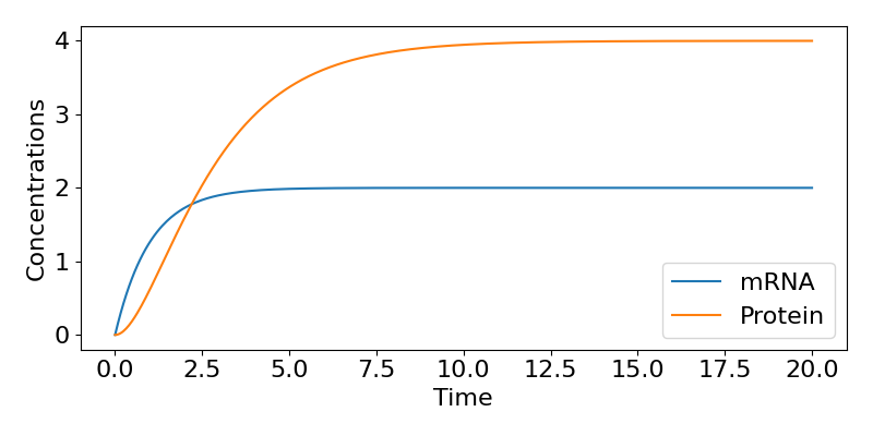
So, in this model, even when we started with 0 concentrations of both mRNA and protein, both eventually tend towards equilibrium values, with the speed of that approach largely dictated by the mRNA degradation rate.

Oscillating transcription

We allowed that the transcription rate, [latex]R(t)[/latex], might depend on time but then just assumed it was constant. What if we instead assume we have an oscillating transcription rate? We will often find that we end up with expressions that are too complicated to integrate explicitly (and in that case we would probably just numerically integrate it on a computer), but if we take a sinusoidal function we can make some progress.

Let’s take the transcription function [latex]R(t)=r_0(1+\delta\sin(\omega t))[/latex]. This has average input [latex]r_0[/latex], but varies between [latex]0[/latex] and [latex]2r_0[/latex], with the period depending on [latex]\omega[/latex]. Returning to our earlier expression, we now need to solve,

[latex]\begin{align} M(t)&=e^{-\mu t}\int e^{\mu t}r_0\left[1+\delta\sin(\omega t)\right]dt\\ &=r_0e^{-\mu t}\left[\int e^{\mu t}dt+\delta\int e^{\mu t}\sin(\omega t)dt\right]. \end{align}[/latex]

The first integral is identical to what we had before, so we can just copy that down again. The second may initially look a bit scary, but is actually quite a classic example of applying the method of integration by parts. This is sometimes called a “product rule for integration”, with the trick being that when you have an exponential multiplied by a sine or cosine, after a couple of steps you get the same integral back again (if you do not know how to do this, you could try asking a friendly mathematician to talk you through it, or look it up online, but we will also go through it in some detail in the exercise solution).

We now need to complete this solution by adding in the initial condition. If we again take the initial condition that [latex]M(0)=0[/latex], you should be able to show that,

[latex]\begin{equation*} C=\frac{\delta\omega}{\mu^2+\omega^2}-\frac{1}{\mu}, \end{equation*}[/latex]

which leads us to the final – somewhat long – solution,

[latex]\begin{equation} M(t)=r_0\left[\frac{1}{\mu}+\frac{\delta}{\mu^2+\omega^2}(\mu\sin(\omega t)-\omega \cos(\omega t))+\left(\frac{\delta\omega}{\mu^2+\omega^2}-\frac{1}{\mu}\right)e^{-\mu t}\right]. \end{equation}[/latex]

As long as this is, it can readily be broken into three parts – a constant term, an oscillating term and an exponentially decaying term. After a long time we can assume the exponentially decaying term stops having much effect, meaning the solution reduces to,

[latex]\begin{equation} M_{long-time}(t)=r_0\left[\frac{1}{\mu}+\frac{\delta}{\mu^2+\omega^2}(\mu\sin(\omega t)-\omega \cos(\omega t))\right]. \end{equation}[/latex]

Using a few more results about trigonometric functions we can reduce this a bit further to,

[latex]\begin{equation} M_{long-time}(t)=r_0\left[\frac{1}{\mu}+\frac{\delta}{\sqrt{\mu^2+\omega^2}}\cos(\omega t-\theta)\right], \end{equation}[/latex]

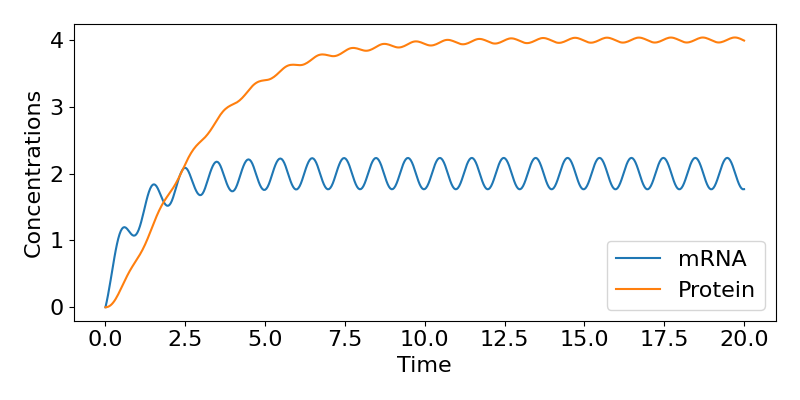
where [latex]\theta=tan^{-1}(\omega/\mu)[/latex]. This then tells us that, in the long-term, the mRNA concentration oscillates around the value of [latex]r_0/\mu[/latex] (the same value as in the constant case), with the same period as the inputted transcription rate (because the ‘time’ term in the cosine is [latex]\omega t[/latex])), but delayed behind the input by amount [latex]\theta[/latex]. We can follow a similar approach to get an expression for [latex]P(t)[/latex] as well if we wish but we won’t cover that here. A time-course of these dynamics is shown below, showing the regular fluctuations in expression.

Chapter references

• The content in the Gene networks section is based on the unpublished Mathematical Biology lecture notes developed by Nick Monk.