A simplified 3-variable model

We saw in chapter 13 that a two-component negative feedback circuit (the auto-repressive gene system) possesses a unique steady state, which is always stable. This underlies homeostasis; the tendency of a negative feedback system to return to its equilibrium when perturbed (for small perturbations, at least).

However, negative feedback circuits can also generate sustained oscillations. One way this can occur is if we extend our two-variable model to a model including at least three variables. This was first proposed in the context of regulated gene expression in the 1960s, and the prototype three-component model is often referred to as the Goodwin oscillator (see chapter references). There are a number of ways of thinking about what might underlie a model of auto-regulatory gene expression that would contain more than two variables. One example would be that in fact the protein product of the gene is translated/produced in one place – the cytoplasm – but regulates transcription in another – the nucleus. We could therefore consider three variables: mRNA, cytoplasmic protein and nuclear protein.

Here, we will look at a slightly simplified model to Goodwin’s original, but the principles remain the same. Rather than focusing on a specific example of gene expression, we will consider a simple model of three interacting components, [latex]X[/latex], [latex]Y[/latex], and [latex]Z[/latex], which form a negative feedback loop by regulating each other. In particular:

• Increasing [latex]X[/latex] leads to increased production of [latex]Y[/latex],
• Increasing [latex]Y[/latex] leads to increased production of [latex]Z[/latex],
• Increasing [latex]Z[/latex] leads to decreased production of [latex]X[/latex].

Put together there is therefore a negative feedback in the system (since increasing [latex]X[/latex] ultimately leads to decreased production of [latex]X[/latex]). For simplicity we will assume that the degradation rates of all three components are the same, so our model can be written as,

[latex]\begin{align} \frac{dX}{dt} &= f_1(Z) - \mu X\\ \frac{dY}{dt} &= f_2(X) - \mu Y\\ \frac{dZ}{dt} &= f_3(Y) - \mu Z. \end{align}[/latex]

Each of the functions [latex]f_i[/latex] are non-negative and bounded as we assumed before. Given our assumptions in the bullet points we also have that [latex]df_1/dZ\lt0[/latex] and [latex]df_2/dx,df_3/dY\gt0[/latex].

Equilibria of this system occur where the following three conditions are simultaneously satisfied:

[latex]\begin{align} & \mu X = f_1(Z)\\ & \mu Y = f_2(X)\\ & \mu Z = f_3(Y). \end{align}[/latex]

How many equilibria can we expect? If we let [latex]F_i=f_i/\mu[/latex], then we have [latex]X=F_1(F_3(F_2(X)))=G(X)[/latex]. We know that [latex]G(X)[/latex] must be a decreasing function of [latex]X[/latex] (intuitively it must be because we know we have a negative feedback loop, but we can also show it by the chain rule). By the same argument as in the two-component auto-repression model, then, we can say that there must be a single equilibrium (because [latex]X[/latex] is an increasing straight line and [latex]G(X)[/latex] is some decreasing function, they can only cross once).

Linear stability analysis

The Jacobian for this system may be 3 dimensional but doesn’t look too horrid,

[latex]\begin{align*} J=&\left( \begin{array}{ccc} -\mu & 0 & \phi_1\\ \phi_2 & -\mu & 0 \\ 0 & \phi_3 &-\mu \\ \end{array} \right), \end{align*}[/latex]

where [latex]\phi_i[/latex] are the derivatives of [latex]f_i[/latex] at the equilibrium point. We have seen before that 3-dimensional Jacobians cannot be solved as easily as other models we have met. However, because we kept this system (relatively) simple we can actually check its stability directly from the characteristic equation, a bit like when we looked at the HIV model. To find this we take,

[latex]\begin{equation} \det(J-\lambda I)=(-\mu-\lambda)^3+\phi_1\phi_2\phi_3. \end{equation}[/latex]

We then look for solutions for [latex]\lambda[/latex] to where this equation equals 0. That is,

[latex]\begin{equation} (\mu+\lambda)^3=\phi_1\phi_2\phi_3=-\chi^30. \end{equation}[/latex] Here we have made the product of our three gradients equal to a new parameter [latex]-\chi^3[/latex]. The minus sign is to remind us that this product is negative (so in fact [latex]\chi\gt0[/latex]) and the cubed is to remind us that this is really the composite of three parameters. The solution to this is then, [latex]\begin{equation} \lambda=(-1)^{1/3}\chi-\mu. \end{equation}[/latex] Somewhat susprisingly then, we find ourselves needing to find the cubed root of -1 in order to understand a real-world biological problem. Recalling that we can write [latex]e^{-i\pi}=-1[/latex] (I bet you didn’t expect to see Euler’s relation in this textbook!), we have that the three possible solutions are,

• [latex]\lambda_1 = -\chi-\mu[/latex],
• [latex]\lambda_2 = e^{i\pi/3}\chi-\mu[/latex],
• [latex]\lambda_3 = e^{-i\pi/3}\chi-\mu[/latex].

We can see that [latex]\lambda_1[/latex] is definitley negative. However the other two eigenvalues are complex, and we can find that they have real part [latex]Re(\lambda_{2,3})=-\mu+\chi/2[/latex]. Putting this all together we find that,

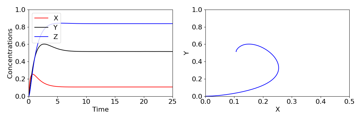
• if [latex]\chi\lt2\mu[/latex], all the eigenvalues have negative real part and the equilibrium is a stable spiral (we know it is a spiral because two of the eigenvalues are complex),
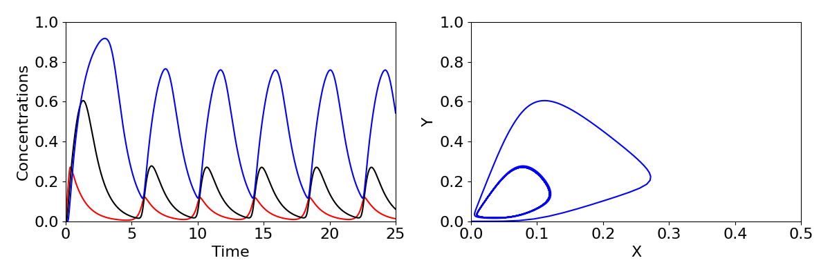
• if [latex]\chi\gt2\mu[/latex], two of the eigenvalues have positive real part and the equilibrium is an unstable spiral.

We have seen a case before where stability moves from a stable spiral to an unstable spiral, when we looked at the predator-prey model. You may recall this produced a Hopf bifurcation, where a limit cycle emerges. The same phenomenon occurs here, with sustained oscillations in the expression of the gene arising. Time-courses and phase portraits of the dynamics before and after the Hopf bifurcation are shown in the figure below, with large oscillations in concentrations shown in the lower plots.

The three-component feedback loop we have considered here demonstrates that negative feedbacks can do more than homeostasis (stability of a system around a fixed point); it can also result in sustained oscillations. Such oscillations are a central feature of many biological systems. A prominent example is the roughly 24-hour period circadian oscillatory gene expression that occurs in both plants and animals. These oscillations, which are critical for coordinating metabolic activity, etc. with the rotation of the Earth, are generated by a slight elaboration of the mechanism we have studied here. Indeed, the Goodwin oscillator provided an early model for studying the properties of circadian oscillations. Other oscillations, with a wide range of oscillatory periods, are also generated by negative feedbacks.

Chapter references

• This model is a simplified version of that proposed by Goodwin (1965).
• The content in the Gene networks section is based on the unpublished Mathematical Biology lecture notes developed by Nick Monk.