Case study: HIV-I

In this chapter we will look at another example of a within-host disease model, and in fact one of the first such models to be developed. Human immunodeficiency virus (HIV) infects immune cells called ‘CD4+ T-cells’, which form an important part of the human immune system. HIV enters these T-cells, replicates within the cell and then releases new virus particles in to the bloodstream. Immediately after first infection, the virus grows rapidly and produces common infection symptoms in the patient. After a few months, these symptoms disappear and the virus concentration reduces to a lower, but steady, level. This ‘asymptomatic period’ can last for years, with the virus density staying roughly constant, and the concentration of T-cells very slowly dropping. Eventually, the T-cell density becomes so low that the patient’s immune system is no longer effective, a condition called aquired immunodeficiency syndrome (AIDS). The patient is then at risk from life-threatening opportunistic infections. From the 1990s, much work has been done to explore the dynamics of HIV and to produce potential treatments, including the development of mathematical models (see chapter references).

A (pre-treatment) model

Let’s start by establishing our variables and drawing a schematic of what is happening in this system. The variables that we want to keep track of (before treatment, at least), are:

• Healthy T-cells ([latex]T[/latex])
• Infected T-cells ([latex]T^*[/latex])
• Virus particles ([latex]V[/latex])

We will only keep track of the concentration of virus particles in the bloodstream, not the ‘intracellular’ concentrations. Our schematic should look like this:

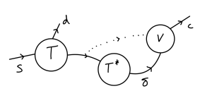
Healthy T-cells are produced at some constant rate [latex]s[/latex] by the body (not a per-capita rate), but also decay at some rate [latex]d[/latex]. These healthy cells become infected through contact with virus, assuming a mass-action process, with coefficient [latex]k[/latex]. These infected T-cells then decay at some rate [latex]\delta[/latex]. New virus particles are produced when infected T-cells die, with [latex]N[/latex] giving the average number of virus particles produced by each cell. The virus then also decays at some rate [latex]c[/latex]. The system can therefore be expressed with the following set of ODEs:

[latex]\begin{align} \frac{dT}{dt} &= s-dT-kVT\\ \frac{dT^*}{dt} &= kVT-\delta T^*\\ \frac{dV}{dt} &= N\delta T^*-cV \end{align}[/latex]

Looking at the equations, we can see that there is an HIV-free equilibrium for [latex](T,T^*,V)=(s/d,0,0)[/latex]. We have another example here of a 3-dimensional system. As we saw in the free-living parasite model, assessing stability here can be a bit more complicated, often reying on using the Routh-Hurwitz criteria. As it turns out, for the HIV-free equilibrium things simplify fairly nicely to the point that we can actually directly calculate one of the eigenvalues, and then just use the trace-determinant conditions (themselves the Routh-Hurwitz criteria for a 2-dimensional system) to determine the sign of the other two.

The general Jacobian is,

[latex]\begin{align*} J=&\left( \begin{array}{ccc} -d-kV & 0 & -kT\\ kV & -\delta & kT\\ 0 & N\delta & -c \end{array} \right). \end{align*}[/latex]

Subsituting in the equilibrium values this becomes,

[latex]\begin{align*} J=&\left( \begin{array}{ccc} -d & 0 & -ks/d\\ 0 & -\delta & ks/d\\ 0 & N\delta & -c \end{array} \right). \end{align*}[/latex]

To find the eigenvalues we want to write out the characteristic equation – the determinant of the matrix of [latex](J-\lambda I_3)[/latex], where [latex]I_3[/latex] is the identity matrix. The characteristic equation is,

[latex]\begin{equation*} (-d-\lambda)\left[(-\delta-\lambda)(-c-\lambda)-\frac{ksN\delta}{d}\right]=0\\ \end{equation*}[/latex]

This is already partly factorised, making our life much easier. The first bracket tells us that one eigenvalue is [latex]\lambda=-d\lt0[/latex]. To find the remaining two eigenvalues we look at what is inside the square bracket, wich can be re-written as,

[latex]\begin{equation*} \lambda^2+(c+\delta)\lambda+\delta c-\frac{ksN\delta}{d}=0\\ \end{equation*}[/latex]

We could use the quadratic formula to solve for the eigenvalues explicitly, but we can also note that this is just the characteristic equation for a two dimensional system, with [latex]-(c+\delta)[/latex] being the trace and [latex]\delta c-\frac{ksN\delta}{d}[/latex] being the determinant. We can then see that we definitely have a negative trace, and that the determinant is positive – meaning the equilibrium is stable – if [latex]c>ksN/d[/latex]. In other words, the decay rate of the virus must be high, and the infection rate and production rate must be low.

Of course, when a patient is to undergo treatment, they will not be virus-free. We are therefore more interested in the pre-treatment infection steady-state, and we will denote these with a subscript 0. Setting the equations for [latex]dT^*/dt[/latex] and [latex]dV/dt[/latex] to zero, yields,

[latex]\begin{equation} N\delta T^*_0=cV_0 \text{ and } kV_0T_0=\delta T^*_0 \implies T_0=\frac{c}{Nk} \end{equation}[/latex]

Solving [latex]dT/dt=0[/latex], then gives,

[latex]\begin{equation} V_0=\frac{sN}{c}-\frac{d}{k} \end{equation}[/latex]

and, by substituting back in,

[latex]\begin{equation} T^*_0=\frac{kV_0T_0}{\delta} \end{equation}[/latex]

We now have expressions for each of these equilibrium values. We won’t prove the stability here as it gets pretty complicated, but it will be stable whenever the infection-free equilibrium is unstable.

Treatment

Assume a patient arrives with their virus and T-cell concentrations at the pre-treatment steady state. We then wish to put them on a course of treatment. There are many different treatments for HIV that act in different ways. We will focus on an early treatment strategy of using ‘protease inhibitors’. These drugs did not prevent infection, but meant that any new virus produced inside infected T-cells were non-infectious. The system therefore becomes:

[latex]\begin{align} &\frac{dT}{dt} = s-dT-kV_IT\\ &\frac{dT^*}{dt} = kV_IT-\delta T^*\\ &\frac{dV_I}{dt} = -cV_I\\ &\frac{dV_{NI}}{dt} = N\delta T^*-cV_{NI} \end{align}[/latex]

Initially this looks like we have made our lives even harder since we now have four equations to deal with! However, it turns out we can simplify things quite a bit. In particular, in the early stages of treatment it is reasonable for us to assume that the number of healthy T-cells stays roughly constant at its pre-treatment level [latex]T(t)=T_0[/latex]. This means [latex]dT/dt[/latex] can be ignored and that [latex]T_0[/latex] can be considered a constant. We also know that before treatment, all virus particles were of the infective type, such that [latex]V_I(0)=V_0[/latex] and [latex]V_{NI}(0)=0[/latex]. If we look at the equation for [latex]dV_I/dt[/latex] we can see it is in fact linear, and since we have just stated what its initial value is, we can solve it fairly quickly using separation of variables.

[latex]\begin{equation} V_I(t)=V_0e^{-ct}\label{vt} \end{equation}[/latex]

Given that [latex]T(t)=T_0[/latex], we now find that [latex]dT^*/dt[/latex] is also now linear,

[latex]\begin{equation} \frac{dT^*}{dt} +\delta T^*= kV_IT_0 \end{equation}[/latex]

It may not initally be obvious that this is linear, since the right-hand side had [latex]V_I\times T_0[/latex]. However, [latex]T_0[/latex] is a constant and we already have an expression for [latex]V_I=V_0e^{-ct}[/latex]. This can therefore be solved using an integrating factor. Let’s go through the working for this.

Taking an integrating factor of [latex]e^{\delta t}[/latex] we can write this as,

[latex]\begin{equation} \frac{d}{dt}\left[T^*e^{\delta t}\right] = kV_0T_0e^{-ct}e^{\delta t} \end{equation}[/latex]

Integrating both sides with respect to [latex]t[/latex] we then get,

[latex]\begin{equation} T^*e^{\delta t} = \frac{kV_0T_0}{\delta-c}e^{-ct}e^{\delta t}+C \end{equation}[/latex]

where [latex]C[/latex] is a constant of integration. After rearranging we reach our initial result,

[latex]\begin{equation} T^* = \frac{kV_0T_0}{\delta-c}e^{-ct}+Ce^{-\delta t}. \end{equation}[/latex]

Earlier we found the pre-treatment equilibrium for [latex]T^*_0=kV_0T_0/\delta[/latex], so we can say that when [latex]t=0[/latex] we have,

[latex]\begin{equation} \frac{kV_0T_0}{\delta} = \frac{kV_0T_0}{\delta-c}+C. \end{equation}[/latex]

We then rearrange to find the constant,

[latex]\begin{equation} C=\frac{-ckV_0T_0}{\delta(\delta-c)} \end{equation}[/latex]

and then substitute back in to get our final solution,

[latex]\begin{equation} T^*(t)=\frac{kT_0V_0}{\delta(\delta-c)}\left(\delta e^{-ct}-ce^{-\delta t}\right). \end{equation}[/latex]

Phew! Now it’s your turn….

This can be added to the solution for [latex]V_I(t)[/latex] to find the overall density of virus particles in the bloodstream at any time point after treatment has begun. After estimating the values of each of the model parameters, researchers plotted the model’s predictions against data of individual patient’s virus concentrations, and found that that the model provides a remarkably good fit. So even though we have a very simplified model of HIV and immune cell interactions and the effects of treatment, we can get useful and applicable insights.

Chapter references

• This chapter is based on models by Perelson and Nelson (1999).