A general model form

In the previous genetic models we have assumed that one gene exists in isolation and its expression is controlled by its ‘own’ mRNA and protein concentrations. Now we will extend our model to look at two interacting genes. The central property of the circuit is that of cross-repression: the product of gene 1 represses the transcription of gene 2, and vice versa.

We will take a fairly general model set-up of two interatcing genes. To keep things a bit more simple we will assume that the two mRNAs have the same degradation rate as each other, that the two proteins have the same degradation rate as each other, and that the functions describing the two transcription and translation terms are identical, then we can represent the cross-repression circuit by the following four ODEs:

[latex]\begin{align} \frac{dm_1}{dt} &= f(p_2)-\mu m_1\\ \frac{dp_1}{dt} &= km_1- \nu p_1\\ \frac{dm_2}{dt} &= f(p_1)-\mu m_2\\ \frac{dp_2}{dt} &= km_2- \nu p_2. \end{align}[/latex]

where [latex]\mu[/latex] and [latex]\nu[/latex] are the degradation rates of the mRNA and protein, respectively, [latex]k[/latex] is the per capita translation rate, and [latex]f(p)[/latex] is a monotonic decreasing function representing regulated transcription. Note that we have assumed such a high degree of symmetry in the equations only for notational and algebraic simplicity; the behaviour that we will study applies also to non-symmetrical models. Even with these simplifications, we are still faced with a 4-dimensional system to analyse! As we will see below, however, if we think about the problem in the right ways we can still gain considerable insight.

Linear Stability analysis

One particular issue with having a four-dimensional system is that it is impossible to sketch out a phase portrait. Instead we will proceed for now by linearising around the equilibria to assess stability. If we set each of the four ODEs to 0, we reach the following expresisons for equilibria,

[latex]\begin{align} &\frac{\mu\nu}{k}p_1=f(p_2)\\ &\frac{\mu\nu}{k}p_2=f(p_1). \end{align}[/latex]

Since [latex]\mu[/latex], [latex]\nu[/latex] and [latex]k[/latex] are positive constants, we can think of this as roughly giving us two expressions, [latex]p_1=cf(p_2)[/latex] and [latex]p_2=cf(p_1)[/latex]. Since [latex]f(p_i)[/latex] is positive but decreasing, if we take our standard sigmoidal shape of regulation function (i.e. a Hill function), we have two general scenarios that can occur here. Below we plot an example of the curves these produce with [latex]p_2[/latex] as a function of [latex]p_1[/latex].

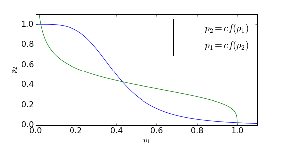
Each curve is a continuum of points along which two of the ODEs are zero. Therefore equilibria of our system occur where these two curves intersect. As such we either have just one equilibrium (where [latex]p_1=p_2[/latex] – and [latex]m_1=m_2[/latex] – because of the symmetry we’ve assumed) or, as we have in the example here, three equilibria (one at [latex]p_1=p_2[/latex] and another two either side of this). As ever, we assess the stability of this system by considering the Jacobian matrix.

We ave seen that with a 3×3 Jacobian, if it is not too complicated, we can still assess stability by writing out the characteristic equation. The same holds here with our 4×4 Jacobian. Thankfully we have a large number of 0s, and we can find that the characteristic equation reduces to,

[latex]\begin{equation} \det(J-\lambda I)=(\nu+\lambda)^2(\mu+\lambda)^2-k^2\phi_1\phi_2. \end{equation}[/latex]

Similarly to last time let us take [latex]\chi=\sqrt{\phi_1\phi_2}[/latex]. Then we are looking for solutions of,

[latex]\begin{align} &(\nu+\lambda)(\mu+\lambda)=\pm k\chi,\\ \implies & \lambda^2+(\mu+\nu)\lambda+\mu\nu\pm k\chi=0 \end{align}[/latex]

We are therefore reduced to a quadratic equation, which we can solve in the standard way, finding,

[latex]\begin{equation} \lambda = \frac{-(\mu+\nu)\pm\sqrt{(\mu+\nu)^2-4\mu\nu\pm 4k\chi}}{2} \end{equation}[/latex]

These eigenvalues may or may not be complex. The important aspect for stability is what happens to the real parts of the eigenvalues. Provided [latex]k\chi\lt\mu\nu[/latex], we must have negative real parts for all four eigenvalues (because the square root is definitely no bigger than [latex]\mu+\nu[/latex]). However, if [latex]k\chi\gt\mu\nu[/latex] and we take the ‘+’ term outside the square root and the ‘+’ term inside the square root, the eigenvalue will be positive (and entirely real).

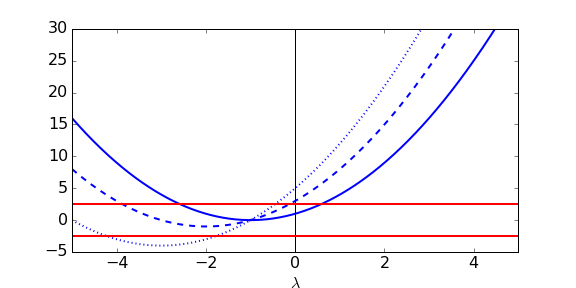
We can try and understand what is going on here a bit more by sketching out the equation [latex](\nu+\lambda)(\nu+\lambda)=\pm k\chi[/latex], as below. In each case we plot [latex](\mu+\lambda)(\nu+\lambda)[/latex] in blue as a function of [latex]\lambda[/latex] and look for where it intersects the red lines for [latex]\pm k\chi[/latex], which will be solutions to our characteristic equation. Notice that [latex](\mu+\lambda)(\nu+\lambda)[/latex] intersects the vertical axis at [latex]\mu\nu[/latex]. We have three cases:

1. The two curves intersect twice (solid blue curve), once for [latex]\lambda\lt0[/latex] and once for [latex]\lambda\gt 0[/latex]. We can see from the plot that in this case [latex]\mu\nu\lt k\chi[/latex]. The other two eigenvalues must be complex (but we know they have negative real part from above).
2. The two curves again intersect twice (dashed blue curve), but now [latex]\lambda\lt0[/latex] at both crossing points. We can see that in this case [latex]\mu\nu\gt k\chi[/latex]. Again, the other two eigenvalues must be complex but we know they have negative real part.
3. The two curves intersect four times (dotted blue curve), and in each case [latex]\lambda\lt0[/latex]. We therefore have 4 purley real eigenvalues. Some further work can reveal that the transition between cases 2 and 3 occurs at [latex]k\chi=(\mu-\nu)^2/4[/latex].

Putting this all together, then, we can either have 4 eigenvalues with negative real parts and so a stable equilibrium (when [latex]\mu\nu\gt k\chi[/latex]), or 3 eigenvalues with negative real parts but one with positive real part and so an unstable equilibrium (when [latex]\mu\nu\lt k\chi[/latex]).

Linking to the equilibria

The challenge now is to work out how each of these cases for stability links to the equilibria we identified earlier. Consider the curves we sketched out in the first figure. Let us think about the respective slopes of the red and blue curves,

[latex]\begin{align} &\frac{dp_2}{dp_1}=\frac{\mu\nu}{k\phi_2}\\ &\frac{dp_2}{dp_1}=\frac{k\phi_1}{\mu\nu}. \end{align}[/latex]

In our first case (one equilibrium), we see the red curve is steeper (more negative) at the crossing point, meaning,

[latex]\begin{equation} \frac{\mu\nu}{k\phi}(k\phi)^2\implies\mu\nu\gt k\chi. \end{equation}[/latex]

(Notice we know that [latex]\phi_1=\phi_2=\phi[/latex] at this equilibrium because of the symmetry. We also change the sign in the inequality because [latex]\phi\lt0[/latex].) We know from above that [latex]\mu\nu\gt k\chi[/latex] means that the equilibrium is stable.

We can see that in the second case (three equilibria), at the two non-central equilibria the red line is again steeper. By the same arguments we can conclude that these two cases will both be stable (although [latex]\phi_1\neq\phi_2[/latex], our definition of [latex]\chi=\sqrt{\phi_1\phi_2}[/latex] is enough). At the central equilibrium we now have that the blue line is steeper. This means our inequalities all reverse and we find that now [latex]\mu\nu\lt k\chi[/latex]. As we found above, this means that this central equilibrium is unstable.

Biological significance

We often find mutually repressing genes in cells. Our modelling shows that if the cross-regulation is weak, or the gene products are stable, then the first case holds, and the two genes weakly hold each other in check, resulting in steady, intermediate expression of both genes.

However, if for some reason either (a) the cross-regulation becomes stronger ([latex]\phi[/latex] increases), or (b) the gene products become destabilised ([latex]\mu[/latex] and/or [latex]\nu[/latex] decrease), then the stalemate state can become unstable, and the second case holds. Now the stalemate state behaves locally like a saddle point, and the state of the system is driven to one of the two new equilibria. In these states, one or the other of the two genes “wins”, and becomes expressed strongly, while expression of the other gene reduces to a low level. The cell has thus switched its gene expression state to either (A ON, B OFF) or (A OFF, B ON). Once one of these states is reached, the system is stable to perturbations.

Such switching of gene expression underlies the basic “fate” decisions that cells have to make during processes such as embryonic development. Since the two protein products of the genes are transcription factors, they can regulate other genes. In this way, a single toggle switch can result in the switching on or off of large collections of genes in a cell, giving coherent choices between different cell fates.

Chapter references

• The content in the Gene networks section is based on the unpublished Mathematical Biology lecture notes developed by Nick Monk.