
3 Thermal comfort, behavioural adaptation and overheating
Analytical and adaptive approaches
As noted in Chapter 1, at its most primitive level, the purpose of a building is to provide shelter, to protect its occupants from climatic extremes and to support them in the attainment of thermal comfort. Our understanding of what constitutes thermal sensation and thermal comfort has evolved significantly during the past 50 years when the pioneering work of Prof. Ole Fanger (1972) became enshrined in the ISO Standard 7730 (ISO, 2005). This standard describes a steady-state heat balance model that translates the rate of heat loss or gain from/to a modelled human body into an average thermal sensation (ranging from cold (-3) through neutral (0) to hot (+3)), the predicted mean vote (PMV), based on feedback from college students that were subjected to a range of conditions in a thermal comfort chamber. In the decades that followed, it became apparent that in what we call free-floating environments that are not maintained at a constant thermal state (of air and radiant temperature, relative humidity and air velocity) the steady-state assumption breaks down so that predictions can deviate significantly from observations. This is particularly the case when occupants have the ability to adapt their circumstances, by adjusting their personal characteristics (clothing level, location, posture, activity level, consuming drinks), the building envelope (window openings, shading devices) or the use of local controls (desk or ceiling fans, local heating or cooling devices). These adaptive behaviours lead to physical, physiological and even psychological feedback that is not accounted for in the PMV model. This has led to a large number of adaptive models being published, mostly predicting a neutral temperature (the temperature that typically corresponds to a neutral thermal sensation vote) based on some average or running mean of outdoor temperature. The supposition here is that indoor thermal conditions are a consequence of the simultaneous outdoor conditions, as are occupants’ choices such as the level of clothing that is selected on a given morning. However, these simplistic models lead to the unintuitive conclusion that the occupants of a highly glazed and poorly ventilated south-facing (in the northern hemisphere) office would experience a similar thermal sensation (neutral temperature) as the occupants of a well ventilated north-facing office in the same location. In response to this illogical conclusion, a large number of models have been developed to predict occupants’ adaptive behaviours and, to some extent, the ways in which these behaviours feedback onto occupants’ thermal sensation and perception of comfort.
But this is only part of the picture. Whilst it is undeniable that we occupants of buildings respond, through our judgements of thermal sensation (from hot to cold), thermal comfort (from comfortable to uncomfortable) and thermal preference (whether we want warmer, the same or cooling conditions) and our decisions to adapt our circumstances as a result, this does not necessarily enable us to make judgements about whether a building’s design has delivered conditions that are generally acceptable; whether a building has delivered indoor conditions that were consistently comfortable, or whether there were too many instances in which the indoor environment was too warm or too cool. This requires the ability to anticipate the indoor thermal conditions over a sustained period of time, and how a population maps these conditions onto a perception of whether a space has under-heated or over-heated; whether their tolerance to cool or warm conditions has been exceeded. In short, a model to predict under-heating or over-heating risk.
In this chapter, we explain each of these concepts and the methods by which they may be evaluated, to support the design of thermal environments in buildings that promote satisfaction amongst their occupants.
3.1 Heat exchange and thermoregulation
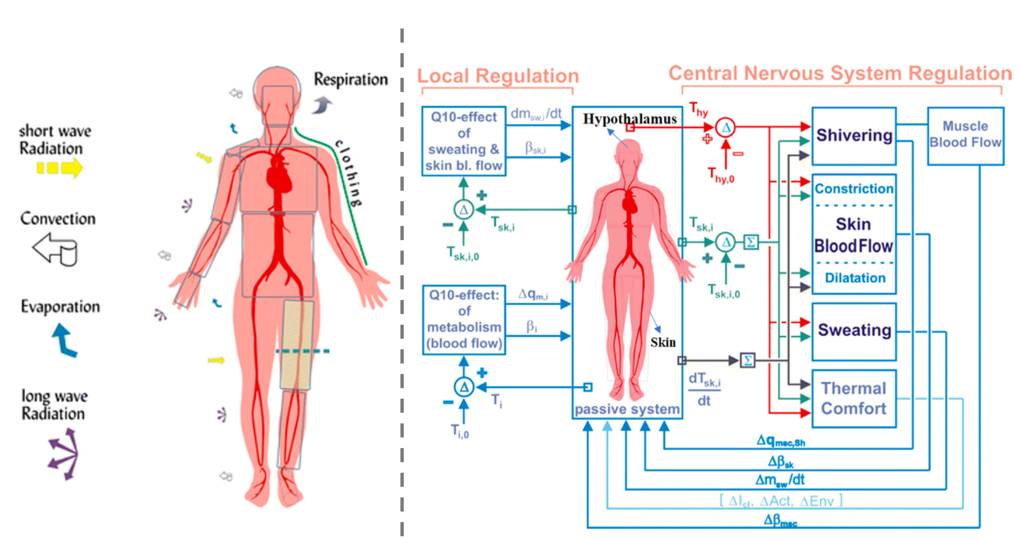
It is estimated that around 60% of human calorie expenditure (Popson et al, 2022) is due to the maintenance of the body’s core temperature, at around 37oC. This involves the metabolism – extracting energy from the chemical bonds – of food to balance the expenditure of thermal energy by a combination of conduction, convection, radiation and evaporation between the human body and the environment in which it is immersed.
At relatively low ambient temperatures (see Figure 1, below), heat transfer from the human body to the adjacent environment is dominated by radiation and convection, with a comparatively small amount of heat also being transferred by conduction (from the feet when standing, or parts of the body in contact with chairs when seated) and by evaporation (due to respiration and the evaporation of moisture that has diffused through the skin). As the ambient temperature increases, the magnitude of heat transfer reduces and the proportion of heat that is transferred by evaporation increases, so long as the vapour pressure is sufficiently low to permit this mode of heat transfer.

We each have thermal receptors in our skin that provoke electrical impulses to be fired in nerve cells that are transmitted by nerve fibres (or axons) towards the brain. Warm temperature signals are transmitted to the anterior hypothalamus in the brain (Figure 2), whereas cold temperature signals are transmitted to the posterior hypothalamus. When a sensation of excess warmth or coolness is perceived, signals are transmitted to effectors that cause active responses in the form of vasodilation, vasoconstriction, sweating, shivering and non-shivering thermogenesis (this latter resulting from the synthesis of Adenosine triphosphate, ATP) and a change in cardiac rate. Vasoconstriction and vasodilation refer to adjustments of the diameter of blood vessels; the latter increasing their diameter and proximity to the surface of the skin to promote heat exchange, the former reducing the diameter and corresponding proximity to the skin surface. Sweating increases evaporative heat transport from the surface of the body. Thermogenesis is comprised of a combination of the metabolism of ATP and shivering, which involves the conversion of chemical to kinetic energy and a corresponding increase in cardiac rate.
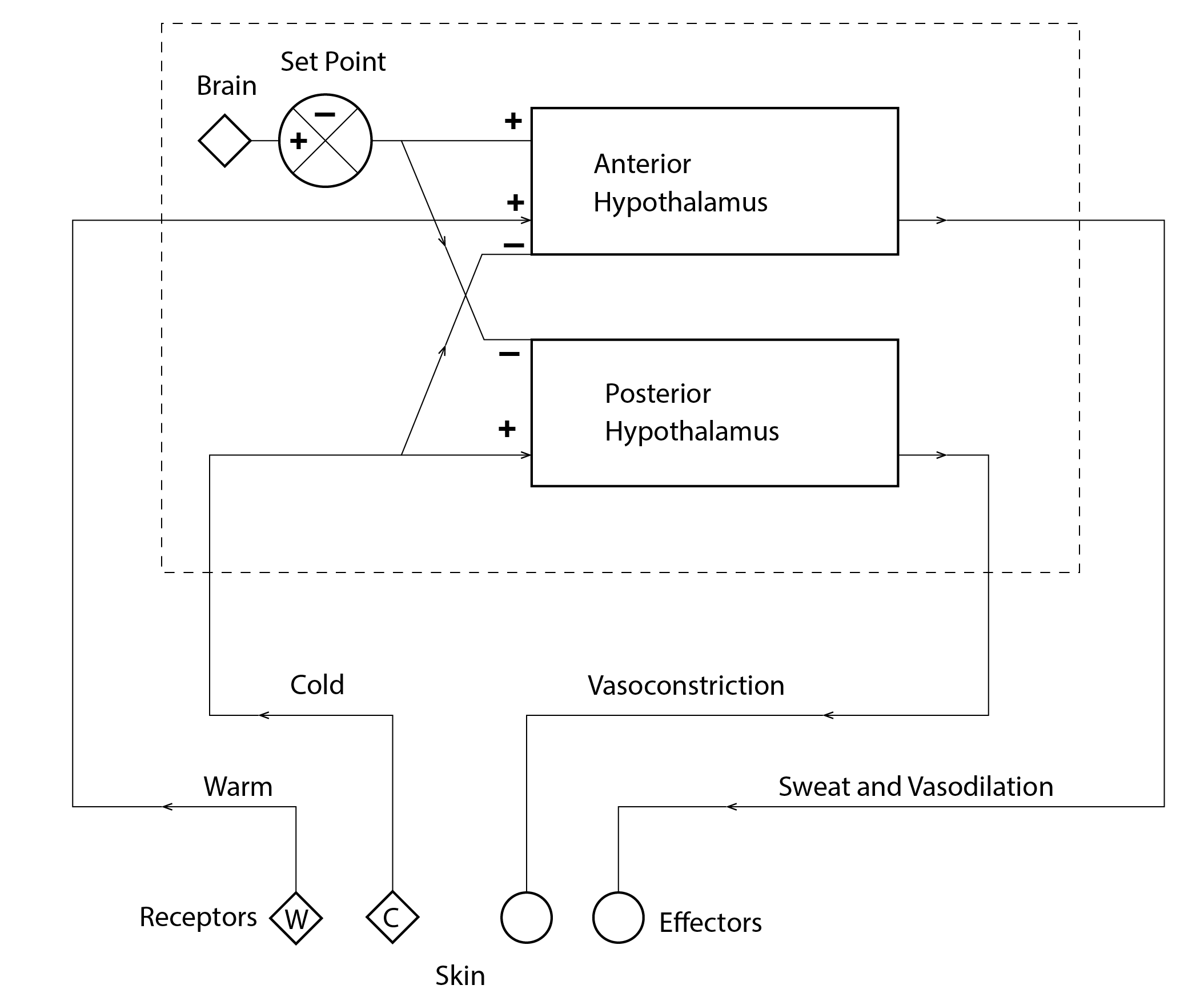
When the core temperature (Tc) becomes elevated ( ) we enter into a state of hyperthermia and, conversely when the core temperature becomes depressed (
 ) we enter a state of hypothermia. Both of these conditions can be fatal. During hypothermia, the body enters into a state of retreat to preserve the functioning of the body’s organs which are critical for life support. As such, the temperature of the extremities (e.g. hands, feet, nose, ears) can be compromised, suffering from frostbite.
3.2 The steady-state heat balance model: PMV and PPD
In the 1970s, the Danish researcher Prof. Ole Fanger (1972) conducted a series of experiments involving College students accommodated in a controlled climate chamber. The conditions in the climate chamber were adjusted to cover a range of air temperature, radiant temperature, air speed and relative humidity. The students were also dressed in attire that ranged from them being naked to heavily insulated and they were also asked to vary their metabolic activity, from sedentary to seated at rest, standing at rest and a range of levels of exercise. Under each scenario, these participants were asked to rate their thermal sensation on a seven-point scale ranging from cold (-3), through cool (-2), slightly cool (-1) and neutral (0) to slightly warm (+1), warm (+2) and hot (+3).
Prof. Fanger (1972) developed a steady-state heat balance model of the human body, calibrating the coefficients of this model so that the mean thermal sensation vote (the Predicted Mean Vote, PMV) matched that which was reported by the study participants. The resultant model (1) and its component parts is presented below.
(1) ![\begin{equation*} \begin{flalign} PMV = (0.303 \exp((-0.036M + 0.028) \cdot \\ [M-W \\ -3.05 \cdot 10^{-3}(5733 - 6.99(M-W)- p_a) \\ -0.42(M-W -58.15) \\ -1.7 \cdot 10^{-5}M(5867-p_a) \\ -0.0014M(34-t_a) \\ -3.96 \cdot 10^{-8}f_{cl}[(273.15+t_{cl})^4 - (273.15 + \overline t_r)^4] \\ -f_{cl}h_c(t_{cl}-t_a)] \end{flalign} \end{equation*}](https://sheffield.pressbooks.pub/app/uploads/quicklatex/quicklatex.com-e25c75b643bf2c8e70b7031ba630c4c4_l3.png "Rendered by QuickLaTeX.com")
This equation (1) is referred to as the PMV model. The above formulation of the PMV model has been split into eight component parts, one per line. The first line (just the right-hand side) represents a coefficient relating to the change in metabolic rate (M). The second line represents heat production in the human body at rest (simply subtracting the work done from the metabolic rate). The third line represents latent heat loss due to the diffusion of vapour through the skin and the fourth line represents latent heat loss due to the evaporation of sweat from the wetted surface of the skin. The fifth line represents heat loss from latent respiration, due to moisture breathed out, and the sixth line is the corresponding heat loss from dry respiration. The seventh line represents radiative heat loss from the clothed surfaces of the body to the bounding environment and the final eighth line represents the corresponding heat loss by convection.
The PMV model requires six parameters, four of which are environmental (the air temperature ta, the radiant temperature tr, the air velocity v – which influences the calculation of the convective heat transfer coefficient hc above – and the relative humidity – which influences the calculation of the water vapour pressure pa above) and two of which are personal (the metabolic rate M and the level of clothing insulation Clo which influences the clothing surface area factor fcl and the clothing surface temperature tcl above). Examples of metabolic rate for different activity levels and clothing insulation Icl for different clothing ensembles are presented in the following tables, reproduced from the ISO standard.
| Activity | Metabolic rate, W/m2 | Metabolic rate, met |
| Reclining | 46 | 0.8 |
| Seated, relaxed | 58 | 1.0 |
| Sedentary activity (office, dwelling, school etc) | 70 | 1.2 |
| Standing, light activity (shopping, laboratory, light industry) | 93 | 1.6 |
| Standing, medium activity (shop assistant, domestic or light machine work) | 116 | 2.0 |
| Walking on level ground:
2 km/h 3 km/h 4 km/h 5 km/h |
110 140 165 200 |
1.9 2.4 2.8 3.4 |
| Work clothing | Icl, clo | Icl, m2K/W | Daily wear clothing | Icl, clo | Icl, m2K/W |
| Underpants, boiler suit, socks, shoes | 0.70 | 0.110 | Panties, t-shirt, shorts, light socks, sandals | 0.30 | 0.050 |
| Underpants, shirt, boiler suit, socks, shoes | 0.80 | 0.125 | Underpants, shirt with short sleeves, light trousers, light socks, shoes | 0.50 | 0.080 |
| Underpants, shirt, trousers, smock, socks, shoes | 0.90 | 0.140 | Panties, petticoat, stockings, dress, shoes | 0.70 | 0.105 |
| Underwear with short sleeves and legs, shirt, trousers, jacket, socks, shoes | 1.00 | 0.155 | Underwear, shirt, trousers, jacket, socks, shoes | 0.70 | 0.110 |
| Underwear with long sleeves and legs, thermo-jacket, socks, shoes | 1.20 | 0.185 | Panties, shirt, trousers, jacket, socks, shoes | 1.00 | 0.155 |
| Underwear with short sleeves and legs, shirt, trousers, jacket, heavy quilted outer jacket and overalls, socks, shoes, cap, gloves | 1.40 | 0.220 | Panties, stockings, blouse, long skirt, jacket, shoes | 1.10 | 0.170 |
| Underwear with short sleeves and legs, shirt, trousers, jacket, heavy quilted outer jacket and overalls, socks, shoes | 2.00 | 0.310 | Underwear with long sleeves and legs, shirt, trousers, v-neck sweater, jacket, socks, shoes | 1.30 | 0.200 |
| Underwear with long sleeves and legs, thermo-jacket and trousers, Parka with heavy quilting, overalls with heavy quilting, socks, shoes, cap, gloves | 2.55 | 0.395 | Underwear with short sleeves and legs, shirt, trousers, vest, jacket, coat, socks, shoes | 1.50 | 0.230 |
This predicted mean vote can be transformed into a predicted percentage of dissatisfied (PPD) individuals, using the following transformation (2):
(2) 
This is expressed graphically in the following chart. Note that the value of the PPD has a minimum at PMV=0 of 5%. This acknowledges the fact that it is not possible to provide thermal circumstances that will satisfy every member of a population. It is not uncommon that air-conditioned environments are regulated to maintain a PMV of ±0.5, corresponding to a PPD of 10%.
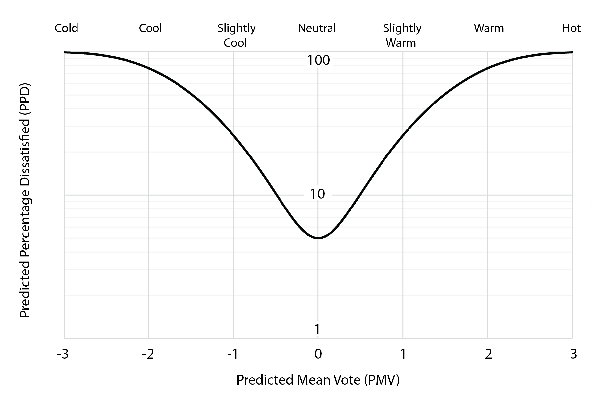
The seven-point predicted mean vote scale has become known as the ASHRAE (American Society of Heating, Refrigerating and Air-conditioning Engineers) seven-point scale of thermal sensation (ANSI/ASHRAE, 2023).
The ISO standard (7730:2005) also contains methods to calculate discomfort due to: draughts, vertical gradients in air temperature, warm or cool floor surface temperatures (which may excessively heat or cool the feet), and radiant temperature asymmetry.
It is worth noting that, as proposed by Griffiths (1990), thermal sensation votes Tsen using the above seven-point scale can be converted into a neutral or comfort temperature (Tc), under the assumption that an increase in indoor air temperature  of 1oC corresponds to a 0.5 increase in thermal sensation, whereby:
(3) 
We will refer to this so-called comfort temperature in section 3.4 when discussing the notion of adaptive thermal comfort. An alternative to this is simply to calculate the mean of the indoor air temperature based on coincident votes of a neutral thermal sensation only, but this tends to require large datasets, since only a fraction of the votes and their coincident air temperatures are processed.
Criticisms of the PMV model
The PMV model assumes that the human body is at equilibrium with the thermal environment. Whilst this is a reasonable assumption in the case of air-conditioned buildings, it is not a safe assumption in the case of free-running buildings. That is, buildings that do not apply energy to maintain a stable indoor thermal environment. Naturally ventilated buildings are one such example. Whilst these buildings utilise heating systems to maintain the indoor environment at or above a set-point temperature during the heating season, they have no such means for regulating the environment during the summertime (the so-called cooling season). Instead, natural ventilation and cooling strategies are employed, often in concert with a variety of opportunities that are presented to the buildings’ occupants to adapt their local environment or their personal circumstances (of which more in section 3.4). Under these adaptive circumstances, the PMV model is considered not to be valid.
Moreover, by modelling the thermal sensation of a population of college-aged individuals, this PMV does not discriminate between age and gender. The metabolic rate of elderly individuals tends to be lower and comfort temperatures correspondingly higher. There are also physiological differences between male and female subjects, which can also have implications for their comfort temperature.
3.3 Dynamic models
Fanger’s (1972) simplified steady-state heat balance model with which to calculate the mean vote of a population and its transformation to calculate the corresponding percentage of dissatisfied individuals came to dominate the discourse of human thermal comfort in buildings for decades. It was also enshrined in an international standard, ISO 7730. However, two other dynamic modelling strategies were developed, both highly sophisticated. A two-node model of human thermoregulation and several yet more sophisticated multi-node models.
Gagge’s two-node model
Gagge et al (1971) developed a dynamic model comprised of passive and active components. The model of the passive system is a relatively straightforward model of human heat balance, of the form:
(4) 
where the term S represents thermal storage, the rate of heating or cooling by the body, M is the rate of metabolic heat production, E is the total evaporative heat loss, R and C are the rates of heat gain or loss by convection and radiation and W is the rate of work that is accomplished. The term E is expanded upon in the model to separately account for latent respiration, vapour diffusion through the skin and the vaporisation of sweat from the skin surface, in much the same way as the Fanger (1972) model in (1). The model accounts separately for the rate of heating/cooling (equation 4) from the core of the body to the skin and from the skin to the surrounding environment.
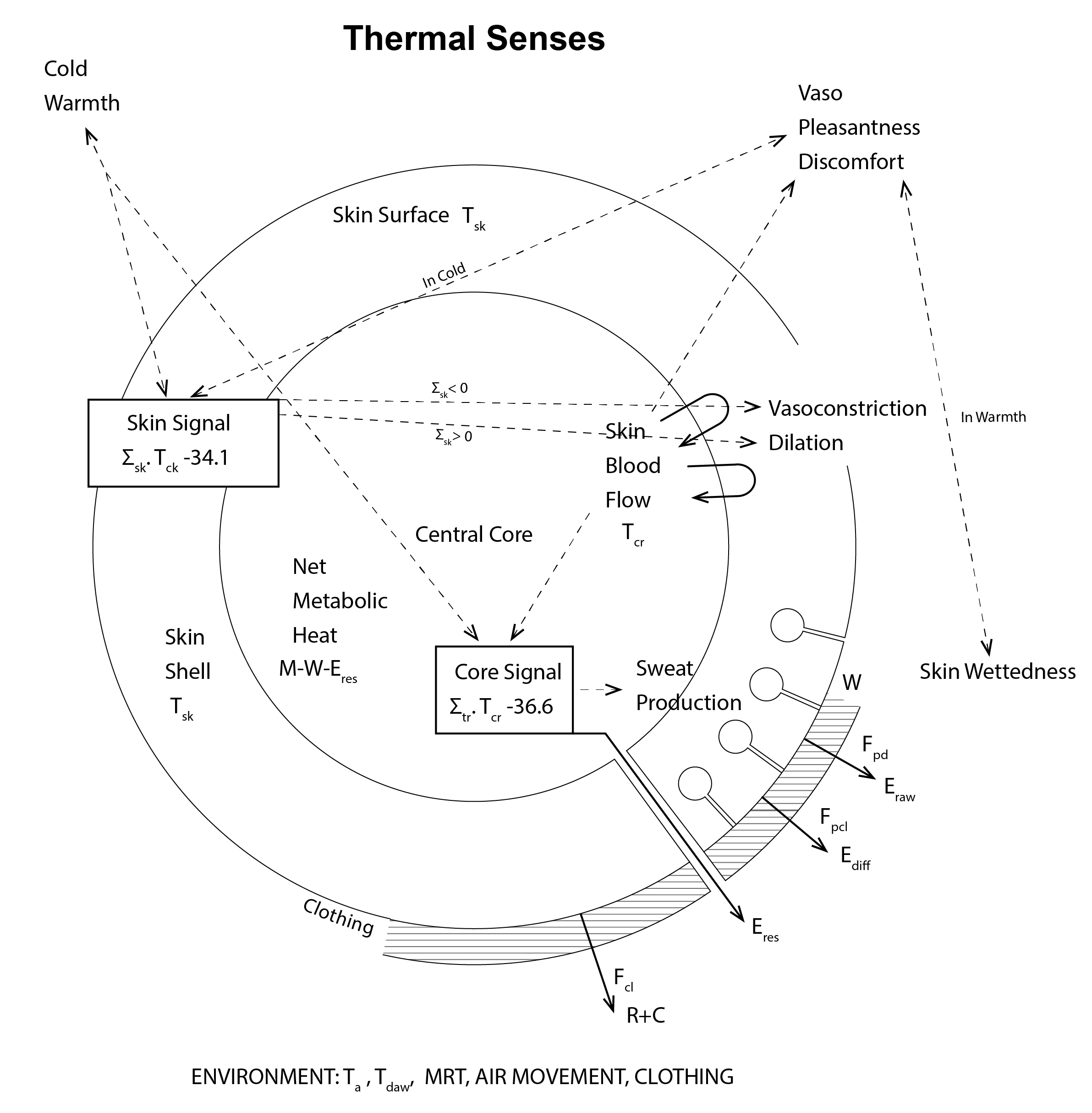
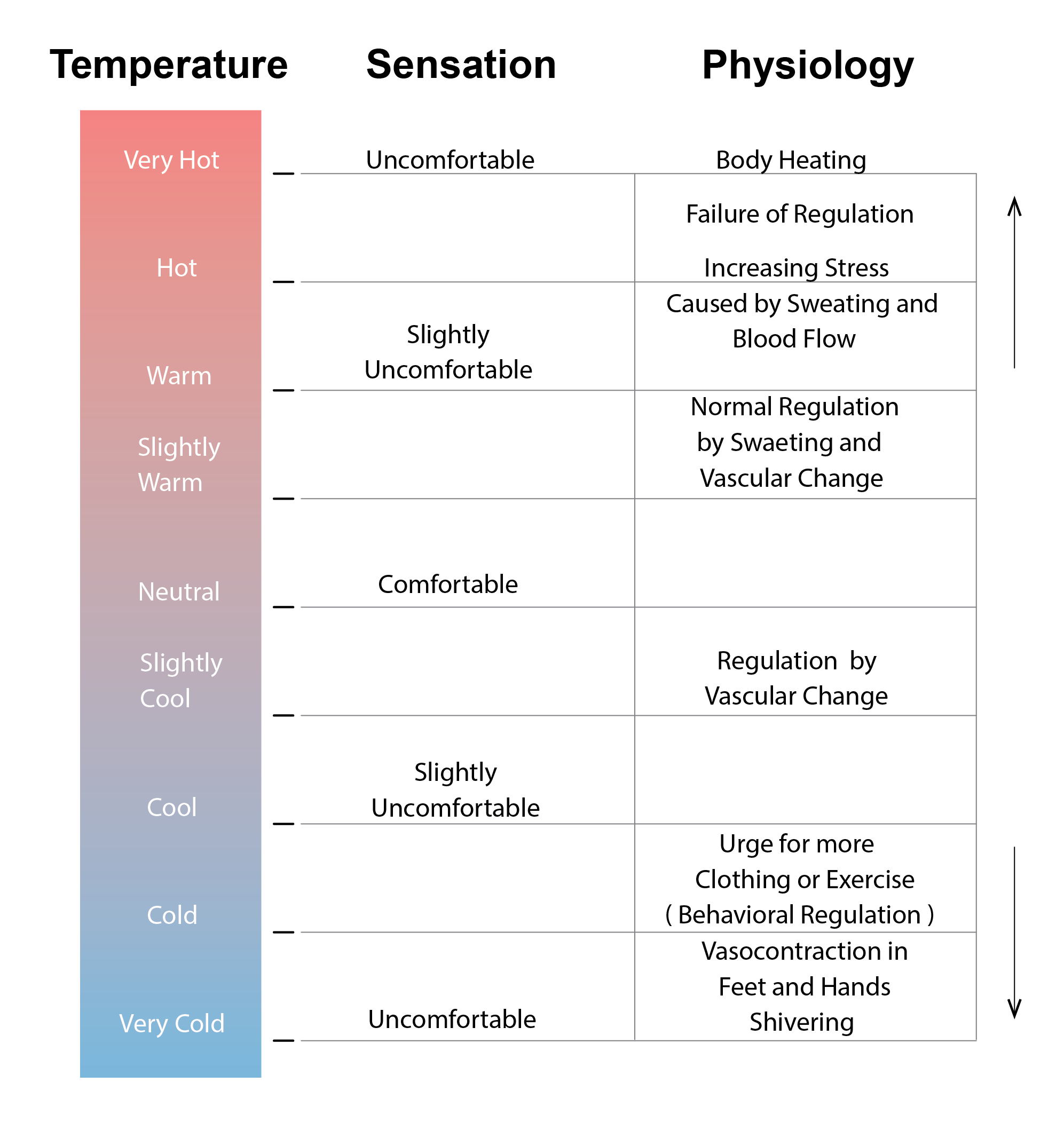
The rates of heat flow for these two nodes are then used, in conjunction with a heat capacity term, to calculate skin and core temperature signals, which are themselves employed to govern an active system of thermoregulatory effector responses, through vasoconstriction, vasodilation and sweating. An effective temperature metric Teff is then calculated (as the loci of dry bulb temperature and 50% relative humidity), which can be mapped onto a thermal sensation, a judgement of comfort and physiological and health responses, as in the following diagram.
Multi-node models
Although both the passive and the active systems of human thermoregulation are represented in Fanger’s (1972) PMV model, this representation is implicit. The active system is explicitly represented in the two-node model of Gagge et al (1971), but this is somewhat incomplete, as it only addresses vascular and sweat-related mechanisms. This is arguably fine when human subjects are situated in near-neutral thermal environments, but is likely to break down at significant departures from these states.
Several multi-node thermal models have been developed in recent years (including those due to Fiala, Tanabe and Zhang – see the review of Zhao et al (2021) for details) which address these shortfalls. The Fiala model – represented diagrammatically in the images below – contains 15 segments, representing the: head, upper and lower abdomen, upper and lower arms, hands, upper and lower legs and the feet. Each of these segments is comprised of three sectors (the anterior, posterior and inferior) and accommodates a range of tissue (brain, lung, bone, muscle, fat, skin and viscera), representing some 187 thermal nodes to account for the transport of heat and mass (in the case of blood and moisture flow). The active system takes temperature signals as an input to regression models derived from empirical data which control the activation of shivering (which also changes cardiac rate), sweating, vasoconstriction and vasodilation.
Predictions from Fiala’s multi-node model compare favourably with observations. The model takes shortwave and longwave irradiance and local relative air velocity and temperature as input, lending itself to the coupling with programs that dynamically simulate indoor microclimates in buildings.
3.4 Adaptive thermal comfort
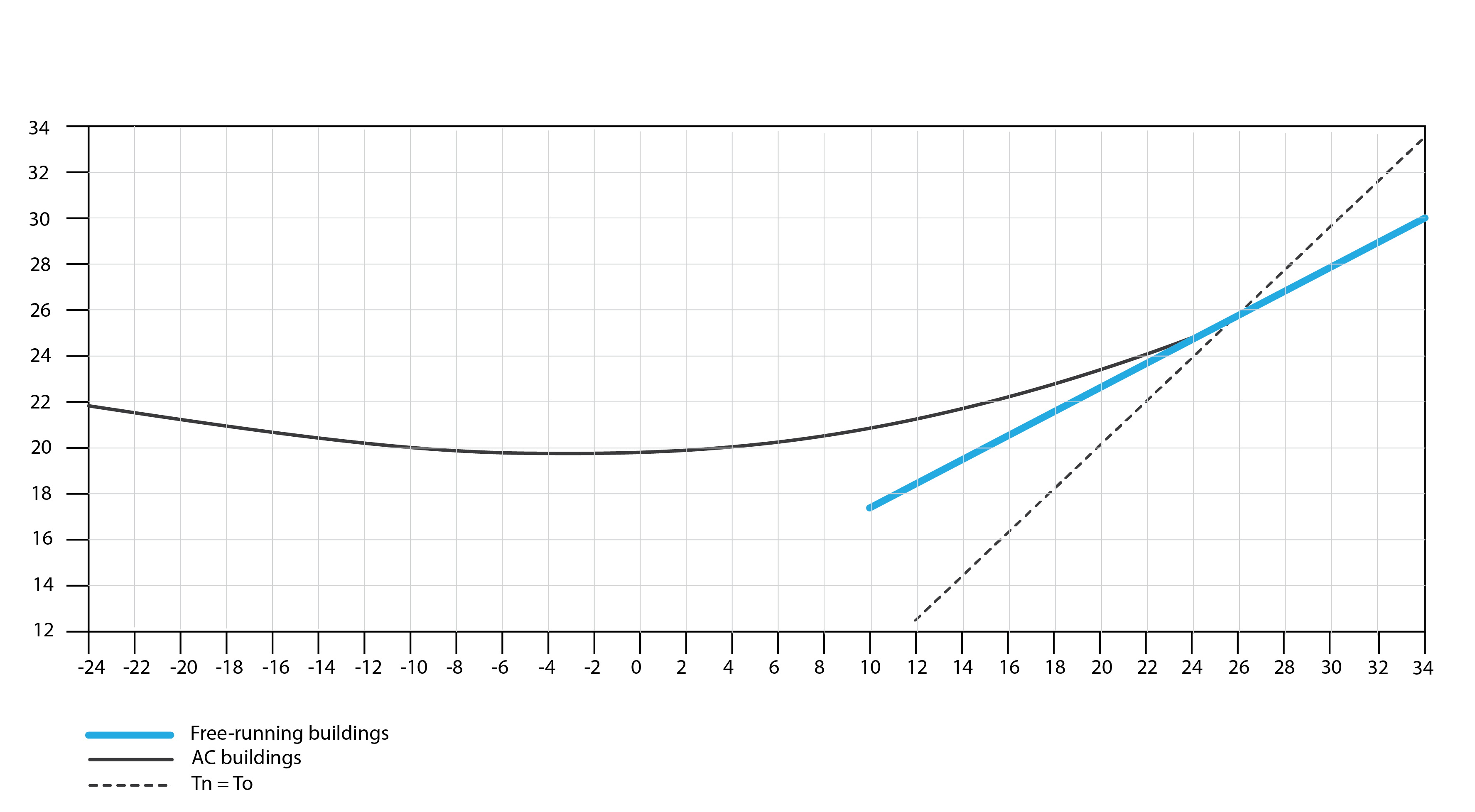
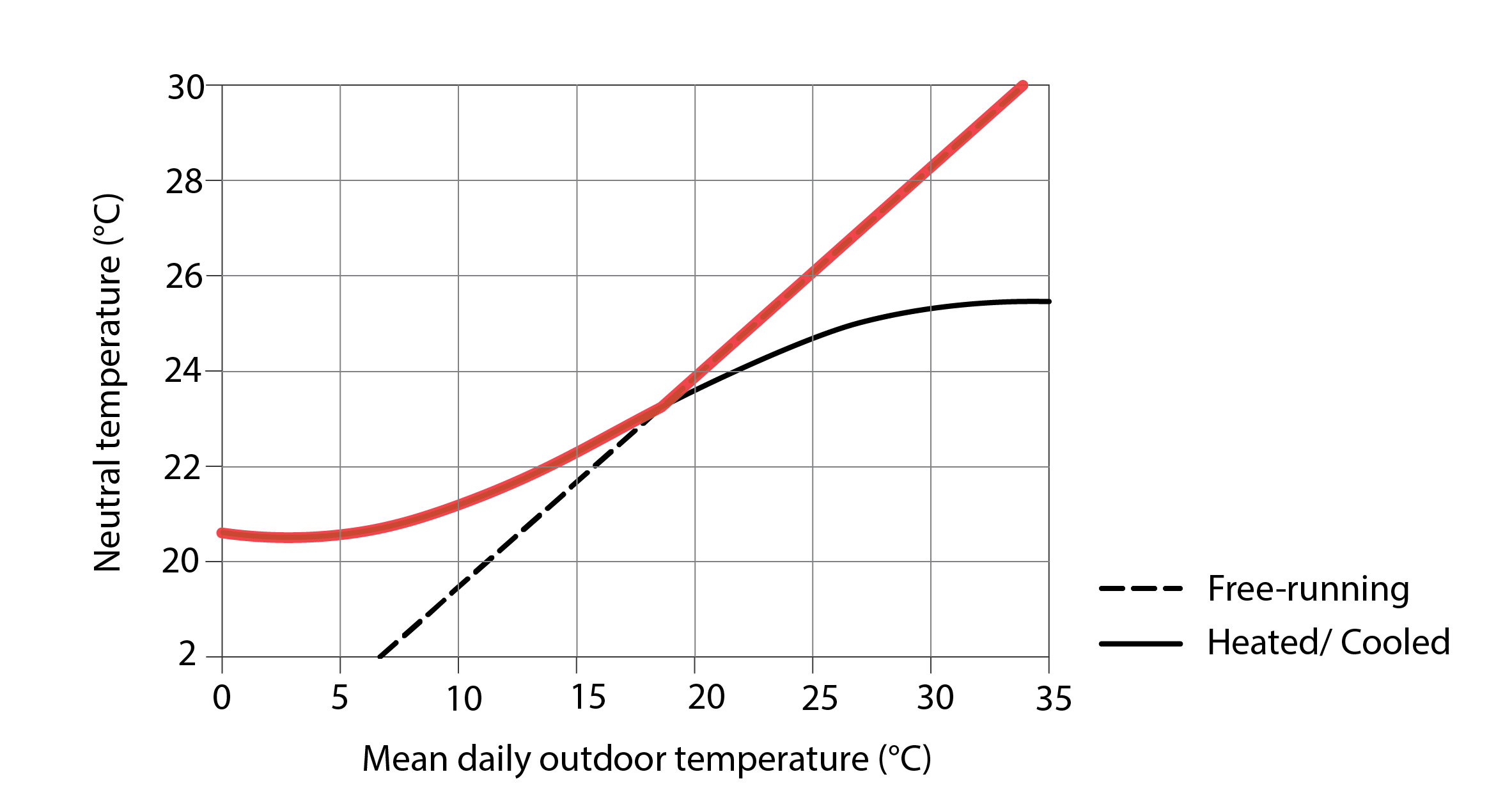
In a seminal paper dating back to 1976, Michael Humphreys (1976) published the first evidence that occupants of free-running buildings have different thermal perceptions and preferences to those of air-conditioned buildings. The graph below compares the neutral temperature calculated from occupants’ thermal sensation votes (the blue line) with a black dotted line in which the neutral temperature is equal to the outdoor temperature. The slope of the former is not as large as the latter, but it is clear that there is a relationship between neutral temperature and outdoor temperature for occupants of free-running (or naturally ventilated and cooled) buildings. It also appears as though this relationship is stronger than for occupants of air-conditioned buildings (represented by the solid black curve), in which summertime indoor temperatures are curtailed through the use of air-conditioning equipment.
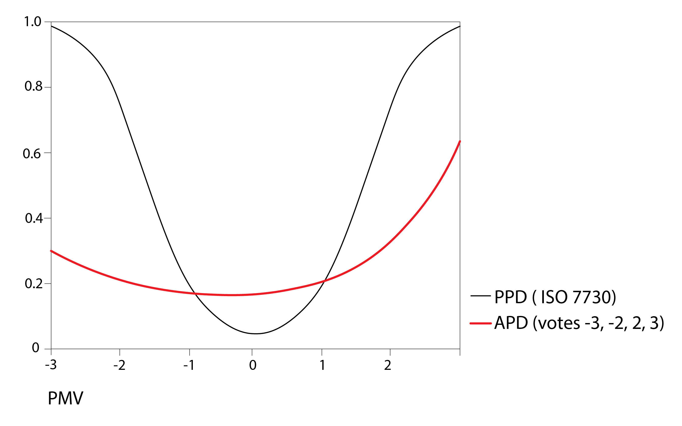
Since this time, a large number of studies have corroborated Humphreys’ findings, including the studies of deDear and Brager (1998) and Humphreys and Nicol (2002), from which the following chart is derived. This chart contrasts predicted mean vote, calculated using the above Fanger (1972) model (equation 1) based on observations of the four physical parameters and the two personal parameters, and the corresponding calculation of the predicted percentage of dissatisfied (PPD) individuals (equation 2), with the corresponding actual percentage of dissatisfied (APD) individuals (the red curve); this latter assuming that votes outside of the thermal sensation range ±2 (i.e. at or beyond cool or warm) correspond to conditions that are regarded as thermally uncomfortable. It is clear from this that there is a significant discrepancy between PPD and APD, again in the case of free-running buildings; that occupants are considerably more comfortable than the PMV model predicts at both the lower and upper bounds of indoor thermal conditions. Something is happening that the PMV model cannot explain.
The primary reason for these discrepancies relates to behavioural adaptation. When the weather has been warm on a particular day and we expect that it will once again be warm the following day, we reduce our clothing level, so that we have less clothing insulation, accordingly. In addition to this planned adaptation, we also react dynamically. This is known as the adaptive principle:
If we are seated at a desk and we perceive our local environment to be uncomfortably warm, we may adjust our clothing level, posture or activity level, switch on a desk fan, open a window, lower a shading device, or consume a cool drink. We call these forms of adaptation our adaptive opportunities, and we exercise these opportunities in an attempt to restore our thermal comfort[1].
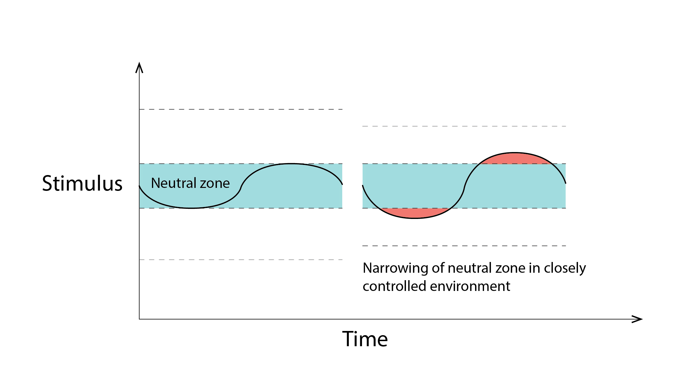
Baker and Standeven (1996) present a series of charts that explain this idea very effectively. The image to the left in the sequence below illustrates a stimulus which varies with time. Let’s assume that this sinusoidal stimulus is thermal in origin, so we have a temperature peak during the afternoon. This stimulus passes through a zone depicted as a Neutral zone, extending above and below this zone during the nighttime and the daytime. Outside of the Neutral zone are two further lines. Baker and Standeven hypothesised that the size of the Neutral zone can be extended by making adaptive opportunities, of the type mentioned above, available to a building’s occupants. Our stimulus magnitude is now contained entirely within this extended Neutral zone. This they thought could explain the deviation between observed and predicted levels of dissatisfaction amongst the occupants of free-running buildings – they are exercising their capacity to adapt and enhancing their comfort as a consequence.
Now if, as in the case of the middle image in the sequence below, the available adaptive opportunities are limited[2] so that the Neutral zone is insufficiently extended, then stress results when the stimulus surpasses this extended zone. If there are no adaptive opportunities, as shown to the right, then stress results whenever the stimulus exceeds the original Neutral zone.
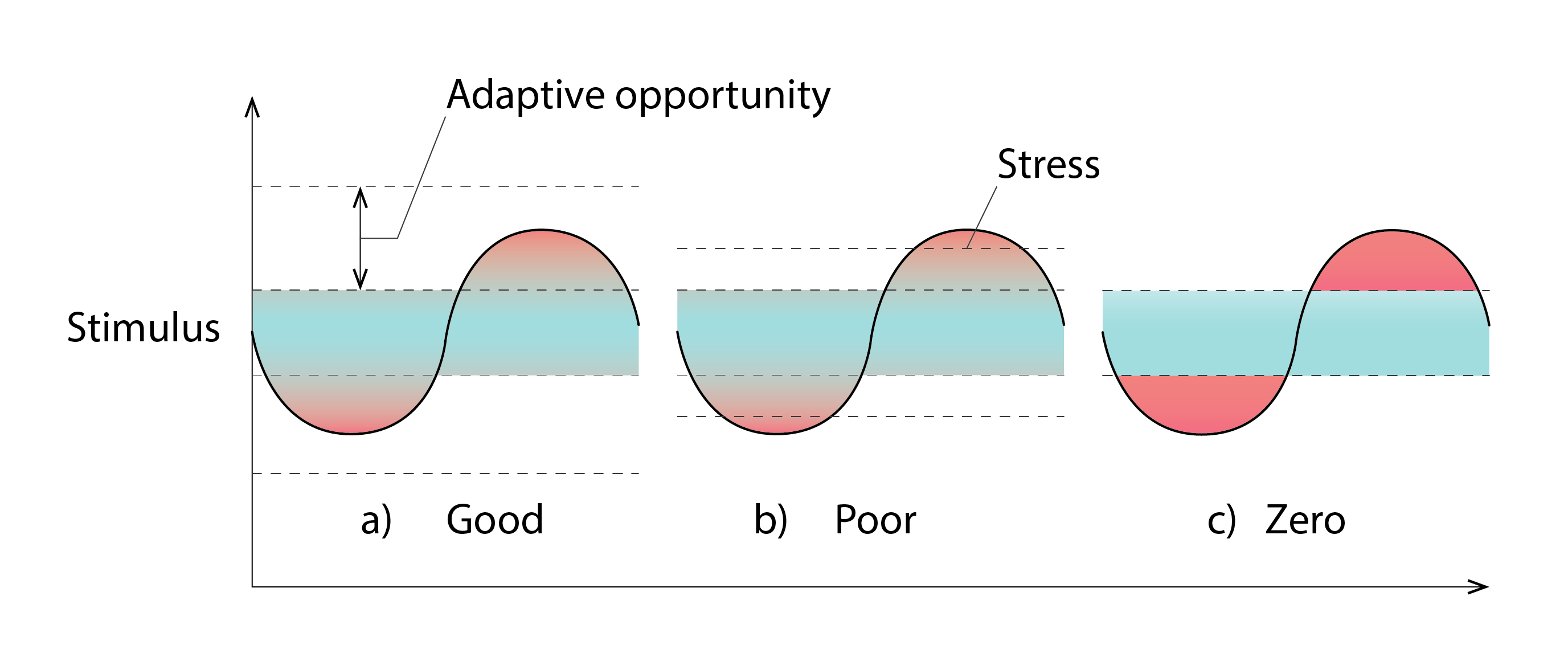
Baker and Standeven further hypothesise that if the magnitude of the stimulus is constrained, so that it does not exceed the limits of the neutral zone (as shown to the left of the image below), then occupants sub-consciously constrict the size of that zone so that they can recover their innate adaptive capacity. At the extreme, with no variation in stimulus, occupants can become hyper-sensitised to other forms of discomfort.
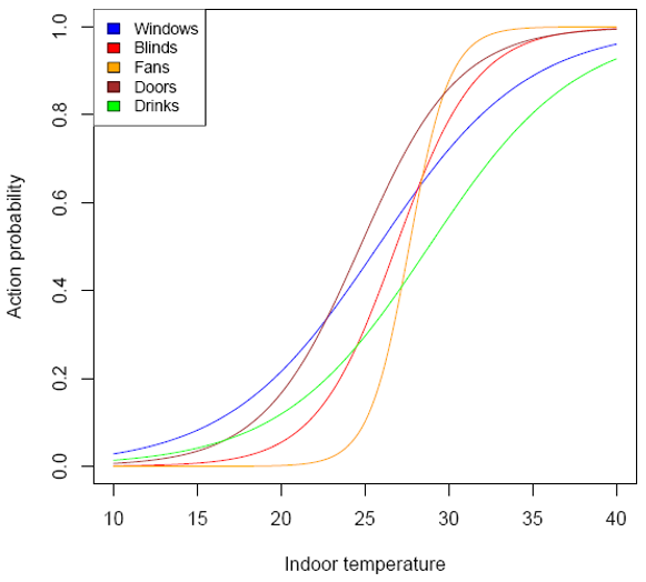
So, do occupants indeed exercise these adaptive opportunities? The answer to this question is an emphatic “Yes”. Indeed the design and execution of field studies into the observation of these adaptive behaviours and the development of statistical models to predict them, has become an intense field of research throughout the past 15 years. One of the earlier studies was that of Robinson and Haldi (2008), from which the following image is derived. This illustrates that, as the local indoor temperature and the corresponding main cause for warm discomfort rises, so too does the probability that occupants of office workplaces will open windows, lower blinds, switch on desk fans if these are available, open doors or drink cold drinks. All to alleviate their discomfort, or rather to restore their comfort.
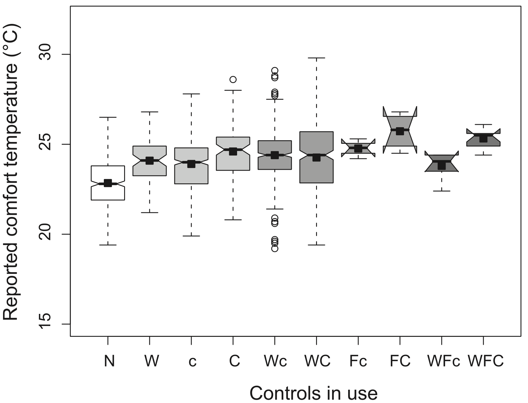
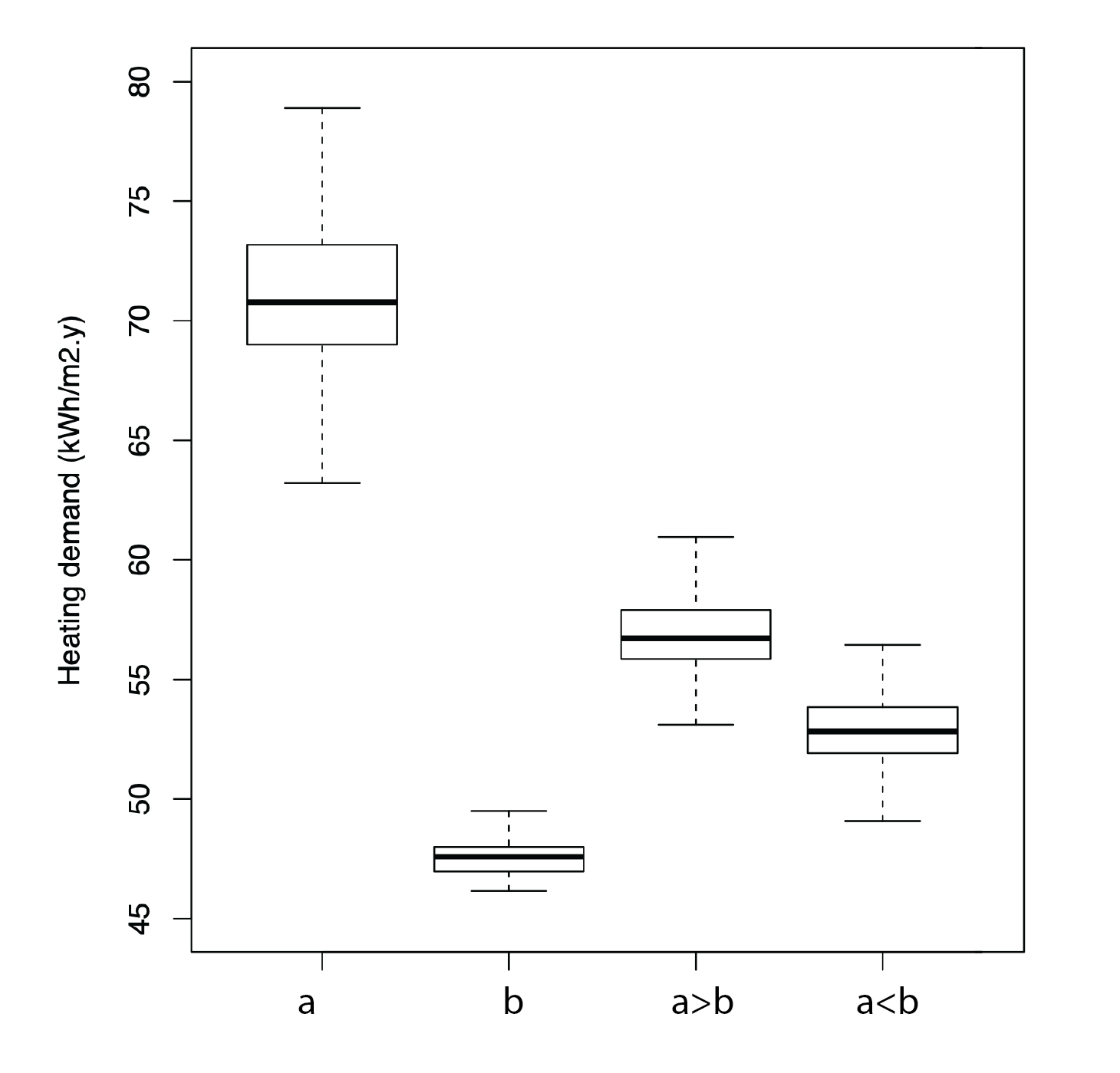
The obvious question, is “Do these adaptive actions really help?”. To shed some light on this, Haldi and Robinson (2008) conducted a field survey (of which more in s 3.5) in which they asked participants to report on whether they had recently exercised any specific types of adaptive opportunity, as well as on their current thermal sensation. These responses were then used to calculate Neutral temperatures (in this case, the temperatures that coincided with Neutral thermal sensation votes, rather than using the Griffiths (1990) formulation, as in equation 3). The chart below presents box plots of Neutral temperature, whereby the upper and lower extremities of the box represents the interquartile range (spanning from the 25th to the 75th percentile), the size of the notch represents uncertainty and the square represents the mean of the Neutral temperature. N, W, c, C and F correspond to No interaction, use of a Window, small and large Clothing level adjustments and Fan interactions respectively and combinations of these represent their conjugates (so that WFc represent the combined interaction with Windows, desk Fans and a small adjustment of clothing level). What is significant here, is that the median (50th percentile) and mean neutral temperatures are consistently higher when an adaptive action (expressed as “Controls in use” in this chart) has been performed than that reported for No interaction. This means that building occupants are comfortable at warmer temperatures when they perform an adaptive action – there is useful and positive feedback. This feedback may be psychological (we have taken ownership of the discomforting influence and performed corrective action, therefore we can tolerate a warmer temperature) or it may be physiological (we have increased the mean air velocity over our skin, increasing physiological cooling, or we have reduced our clothing insulation) or a combination of the two. The important point here is that these results seem to confirm Baker and Standeven’s hypothesis, that the Neutral zone can be enlarged when adaptive opportunities are both available and exercised!
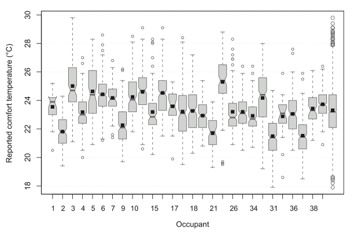
The above results are based on the behaviours and their corresponding feedback for a population of individuals accommodated within different and somewhat unique environments. In reality, however, we humans are all different. We perceive the environment differently from one another and, even when subjected to identical environmental stimuli, we respond differently. Our perceptions and behavioural responses are what we call stochastic in nature. To demonstrate this principle, the box plots in the image below present distributions of Neutral temperature resulting from thermal sensation votes for different individuals. These are all, every single one of them, unique.
In theory, we can develop statistical models that predict the likelihood that individual (or indeed synthetically averaged) occupants will exercise adaptive opportunities and account for both the energy and comfort consequences of these actions. A plethora of such models have been developed in recent years, based on empirical observations, to determine the probability with which occupants will open or close windows, raise or lower shading blinds, switch on fans, adjust heating thermostat settings etc. If we draw a random number and that number is smaller than the probability of a particular behavioural action, then we could infer that that specific adaptive action would be undertaken. For example, we might have a statistical model which predicts that, for an indoor temperature of 25oC there is a 0.65 probability that an office occupant would open a window. If we draw a random number of 0.62, we would then infer that our hypothetical occupant would indeed open their window.
We can also embed these models of occupants’ behaviour within computer programs which generate synthetic populations of agents (computerised versions of people) and assign to these agents models of their adaptive actions and associated feedback. The Nottingham Multi-Agent Stochastic Simulator (No-MASS) is one such example (Chapman et al, 2018). Shown below are four box plots of heating energy use, each produced from 50 repeated hourly simulations of annual heating energy use from a small office building; the only difference between these simulations being that a random number generator was randomly seeded at the beginning of each annual simulation period, so that different actions would be performed by the same synthetic agents even under the same circumstances.
The results for agent “a” relate to someone that frequently opens their window, even when it is relatively cool outside. Agent “b” on the other hand interacts relatively infrequently with their windows, so that the median demand for heating of their office is significantly lower than that of agent “a”. The third box plot results from a situation in which both agents now occupy the same office, but we have allocated to agent “a” more rights to interact than agent “b”. This might for example occur when an employer (“a”) occupies the same office as an employee (“b”), or simply when “b” is more reticent to interact than “a”. The outcome is that the median value from this combined case is, as would be expected, higher than that for the office occupied solely by agent “b”, but it is much lower than that occupied solely by agent “a”. The reason is that agent “b” is sneaky. On many occasions when agent “a” leaves the office (for a separate stochastic model is predicting this event), agent “b” closes the window! As expected, the median energy use is lower still when agent “b” has more voting or action rights.
Despite the significant advances that have been made in thermal comfort and behavioural modelling research, a unification of the joint modelling of these phenomena remains elusive. Indeed, it remains surprisingly commonplace for researchers to estimate so-called adaptive algorithms. These are nothing more than simple linear regression models that estimate the mean Neutral temperature of a population as a function of an average or running mean (as in the case of equation (7) below) of the outdoor air temperature. These models do however have a practical use, in that they can be used to regulate a heating system to reduce energy expenditure during the winter time (as illustrated by the red line in the image below).
However, these models do not predict the actions of specific individuals, accommodated in specific buildings with specific adaptive opportunities available to them and the corresponding feedbacks to their perceived thermal sensation and the mapping of this onto their sense of satisfaction. Achieving this will, in all likelihood, be a long-term endeavour.
3.5 Overheating
There is an important conceptual difference between thermal comfort and the risk of overheating. Thermal comfort relates to a person’s perception of the thermal environment at a specific instant in time. Translating some perceived thermal sensation, as in the ASHRAE seven-point scale, onto a judgement of satisfaction, or comfort. Overheating is different. As hypothesised and demonstrated by Robinson and Haldi (2008a), a space is judged as having overheating when an occupant’s tolerance to uncomfortably warm stimuli has been exhausted; notwithstanding the adaptive opportunities that may have been exercised. This may be thought of as a discharge in tolerance to uncomfortably warm conditions.
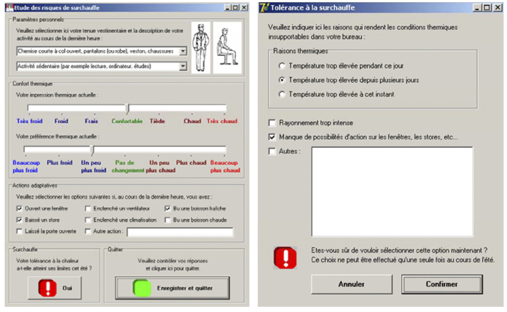
To demonstrate this, Robinson and Haldi conducted a simple experiment within a sample of office buildings located in Switzerland, during the particularly warm summer of 2006. This involved installing a simple electronic questionnaire on the personal computer that was located at the workstation of the study’s participants. In close proximity to their computer, a shielded temperature sensor[3] recorded, on a continuous basis, the local air temperature.
The study participants were asked to complete one questionnaire (shown left below) two to three times per day, as agreed with them, to capture their thermal sensation, thermal preference, clothing and activity levels and any actions that they had undertaken in response to discomforting influences. They were also asked to press, just once, a button to indicate that their tolerance to heat had now been exceeded. This prompted the appearance of the screen shown to the right of the image below, which asked them to explain what caused them to press the ‘overheating’ button. 55% of the participants noted that it was an excess of heat over a period of several days that prompted them to press this button and a further 27% noted that this was prompted by an excess of heat during this particular day. Only 18% of the participants noted that this was caused by the temperature being too elevated at that instant in time.
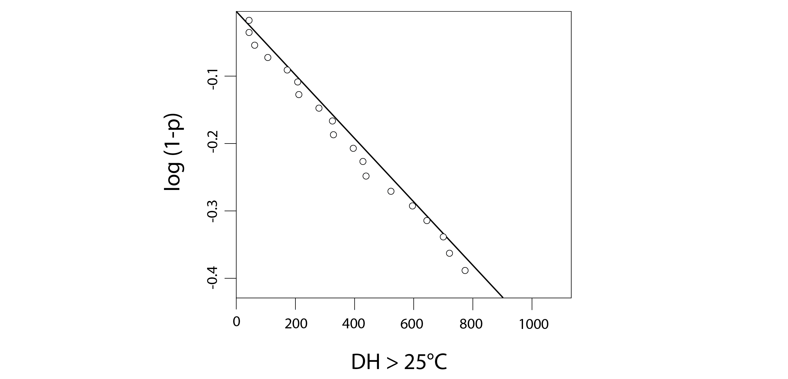
Robinson and Haldi hypothesised that the discharge of tolerance to heat was akin to the discharge of electrical charge from an electrical capacitor (or of heat from a thermal capacitor) and that, during a subsequent cool period, this tolerance could be recharged, owing to the sense of relief following the spell of warm weather. This could take place during the wintertime in readiness for the following summer or simply during a spell of cooler weather following a heatwave. They formulated a model that predicts the likelihood that a population would judge a space to have overheated for a continuous period of tolerance discharge, as a function of the degree-hours of excess of an arbitrary reference temperature, chosen to be 25oC. The form of this model is as follows:
(5) 
where  is a discharging time constant and
  is the cumulative degree-hours of excess of the threshold temperature throughout the period spanning t0 to t. By re-arranging this expression, so that
  , a simple linear regression can be performed (illustrated in the chart below) to estimate the value of this discharge coefficient: the slope of this curve (Fig 17), which gives a value of -4.75×10⁻⁴ (K-1h-1) with very good agreement (r2 = 0.98).
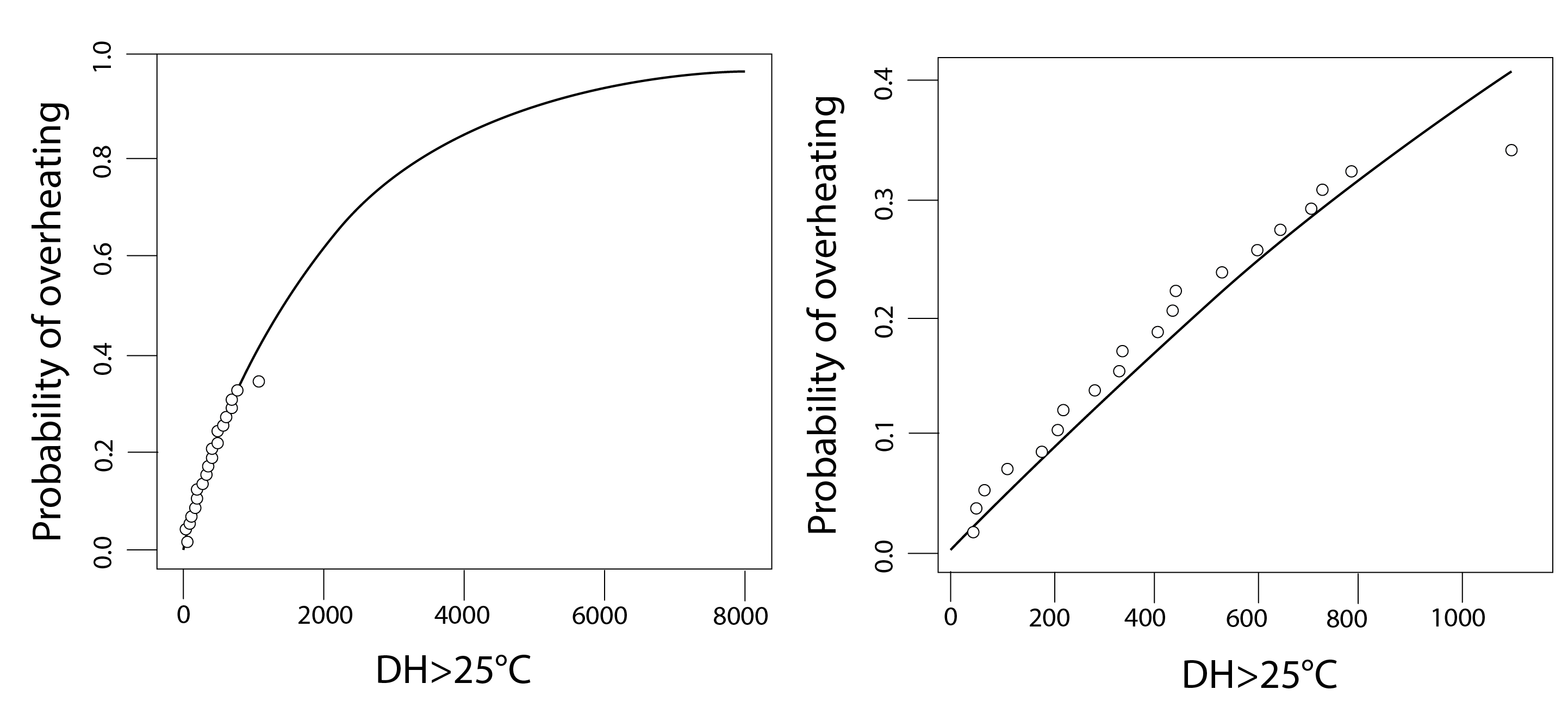
Shown below (Fig 18) is a comparison of the prediction from this simple model (the line) with the reported overheating votes from the study participants (the solid diamonds) – for a range of values of DH > 25oC up to 8,000 (left) and restricted to the range of values experienced during the study: up to 1,200 (right). Both show very good agreement.
This was a useful study, which successfully demonstrated the empirical calibration of a theoretical model to predict the probability with which an indoor environment would be judged to have overheated. The formulation of the model was also extended to account for the feedback of adaptive actions that would act to reduce this probability (Robinson and Haldi, 2008b). However, this model is only applicable to office workplace environments. It cannot be used with confidence to predict the likelihood that a residential space would overheat. This is in part because within our home settings, we have more degrees of freedom with which to adapt our circumstances (clothing, activity level, consumption of food and drink, use of HVAC and envelope controls etc) and in part (indeed the most part) because within our homes we seek to sleep at night time and this quest can be very much compromised during periods of warm or hot weather.
A first attempt to address this was published by the Chartered Institution for Building Services Engineers (CIBSE) in 2005, in the form of Technical Memorandum 36. TM36 contains two overheating criteria for homes. The first states that a threshold temperature for living areas of 28oC should not be exceeded and the second states that a temperature of 25oC should not be exceeded in bedrooms for more than 1% of occupied hours.
These criteria were updated in 2017, in the form of TM59. This states that a temperature difference ( ) between the operative temperature
  and some maximum threshold temperature
  should not be exceeded for more than 3% of occupied hours in living areas and that a limiting temperature of 26oC should not be exceeded for more than 1% of hours, during the period 10 pm to 7 am.
(6) 
where  is an exponentially weighted running mean of the outdoor air temperature:
(7) 
in which  is the mean outdoor air temperature i (= 1, 2, 3…n) days in the past and
  is a constant, with a recommended value of 0.8.
Similar criteria to these were previously proposed for office workplace environments, with the publication in 2013 of TM52. This states that a workplace is deemed to have overheated if any two of the following situations have occurred:
(8) 
Whilst these CIBSE criteria appear to be credible in principle, none of them are based on empirical evidence. Furthermore, they lead to different design outcomes from one another and also with respect to the empirically-based model of Robinson (Gorjimahlabani, 2020). There remains a need for further empirical research in this area, for residential applications in particular.
3.6 Design for comfort
Based on the above, the following principles are recommended for the design of thermal environments that enable occupants to maximise their thermal satisfaction (or to minimise thermal dissatisfaction):
- Provide occupants with effective mechanisms by which to exercise their inherent adaptive capacity, with respect to their personal characteristics (activity, location, clothing level, consumption of warm and cold food and drinks), the envelope of the building (use of windows and shading devices) and the regulation of local and centralised control of heating, ventilating and cooling systems (temperature set-points, use of fans).
- Where building management systems are employed to regulate some or all of the above, ensure that occupants are provided with the means by which these automated control actions may be overridden.
- Avoid environmental conditions that entail strong asymmetry in the radiant environment, strong vertical air temperature gradients, localised draughts (e.g. from open windows above seated locations) and floor surfaces that are excessively warm or cool (see ISO 7730:2005 for more specific recommendations).
- Provide mechanisms by which centralised heating or cooling may be linked with the external temperature, using an adaptive algorithm, to minimise the use of applied energy.
- Ensure that the functioning and control of the indoor environment are readily understood and that this is clearly communicated to the building’s occupants.
- Where feasible, ensure that the performance of the building is evaluated following its occupation, to ensure that it performs as intended and that any deficiencies in this respect can be resolved.
3.7 Questions and worked examples
This section contains a series of worked examples or problems (P) and their solutions (S), as well as a series of written questions (Q) and their written answers (A).
Q1) What are the four physical parameters and the two personal parameters that are used as inputs to the Predicted Mean Vote model?
Q2) What are the four mechanisms of the active system of human thermoregulation?
Q3) What is the distinction between thermal comfort and overheating?
A1) The physical parameters are air temperature, radiant temperature, relative air velocity and relative humidity. The personal parameters are metabolic rate and the level of clothing insulation.
A2) Shivering, sweating, vasodilation and vasoconstriction.
A3) Thermal comfort is an instantaneous response to the thermal environment, whereas overheating results from an accumulation of discomforting influences, until the limit of a subject’s tolerance to these influences has been reached or exceeded.
References
ANSI/ASHRAE (2023), ANSI/ASHRAE Standard 55: Thermal Environmental Conditions for Human Occupancy.
Baker, N.M Standeven, M.A. (1996), Thermal comfort for free-running buildings, Energy and Buildings, 23 p175–82.
Chapman, J., Siebers, P.O., Robinson, D. (2018) On the multi-agent stochastic simulation of occupants in buildings, Journal of Building Performance Simulation 11 (5), 604-621.
CIBSE (2005): TM36 Climate change and the indoor environment.
CIBSE (2013): TM52 The limits of thermal comfort- avoiding overheating.
CIBSE (2017): TM59 Design methodology for the assessment of overheating risk in homes.
deDear, R. & Brager, G. (1998) Developing an adaptive model of thermal comfort and preference. ASHRAE Transactions 104 (1).
Gagge, A.P., Stolwijk, J.A.J. Nishi, Y., (1971) An effective temperature scale based on a simple model of human physiological response, ASHRAETransactions 77 (1) p247–262.
Gorjimahlabani, S. (2020), Evaluation of overheating risk in homes, MSc dissertation, University of Sheffield.
Griffiths I (1990). Thermal comfort studies in buildings with passive solar features, field studies. UK: Report of the Commission of the European Community ENS35 090.
Haldi, F., Robinson D. (2008), On the behaviour and adaptation of office occupants, Building and Environment
43 (12) p2163-2177.
Haldi, F., Robinson, D. (2008a), Model to predict overheating risk based on an electrical capacitor analogy, Energy and Buildings 40 (7), 1240-1245
Haldi, F., Robinson, D., (2010), On the unification of thermal perception and adaptive actions, Building and Environment 45 (11), 2440-2457.
Humphreys, M.A. (1976). Field studies of thermal comfort compared and applied. Journal of the Institute of Heating and Ventilating Engineers, 44, pp 5-27.
Humphreys, M.A. Nicol, J.F (2002), The validity of ISO-PMV for predicting comfort votes in every-day thermal environments, Energy and Buildings, 34(6) p667-684.
ISO (2005), ISO 7730:2005: Ergonomics of the thermal environment: Analytical determination and interpretation of thermal comfort using calculation of the PMV and PPD indices and local thermal comfort criteria.
Popson, M.S., Dimri, M., Borger, J., Biochemistry, Heat and Calories, 2022 (https://www.ncbi.nlm.nih.gov/books/NBK538294/)
Robinson, D., Haldi, F. (2008a), Model to predict overheating risk based on an electrical capacitor analogy, Energy and Buildings, 40 (7), 2008, Pages 1240-1245.
Robinson, D., Haldi (F (2008b), An integrated adaptive model for overheating risk prediction, Journal of Building Performance Simulation, 1 (1), 2008, p43-55.
Zhao, Q., Lian, Z., Lai, D. (2021), Thermal comfort models and their developments: A review, Energy and Built Environment 2, p21–33.
Further reading
Nicol, F., Humphreys, M., Roaf, S. (2012), Adaptive thermal comfort: Principles and practice, Routledge.
McIntire, D. A., Indoor Climate, Applied Science Publishers, 1980.
Fanger, P.O. (1972), Thermal Comfort: analysis and applications in environmental engineering, McGraw-Hill, 1972.
Parsons,L (2003), Human thermal environments, Taylor & Francis (2nd Ed), 2003.
- This dynamic adaptive response to discomforting stimuli to restore thermal comfort is sometimes referred to as thermal alliesthesia, which may also be interpreted as being synonymous with thermal pleasure, since we as a species have evolved to exercise our adaptive capacity and we derive pleasure from doing so. ↵
- An example might be a workplace setting that has somewhat strict requirements regarding attire and posture, where desk fans are not provided and where the windows and shading devices are fully automatically controlled. ↵
- This was nothing more than a temperature sensor that was placed within a polished metallic cylinder, to protect the sensor from the influences of shortwave and longwave radiation exchange. ↵
