Solar geometry and radiation exchange

Darren Robinson

5 Solar geometry and radiation exchange

The energy that we receive on our planet Earth from our Sun is the basis of all of life. It drives photosynthesis and without this abundant source of heat energy, the Earth would be around 30^oC cooler. By effectively harnessing solar energy by passive means, we in the UK can largely avoid the need for additional applied energy to heat our buildings. We can of course also convert solar energy into electrical energy using photovoltaïc panels to power lights, appliances and the technology to heat, ventilate and cool our buildings. It is crucial then that we understand how to exploit this abundant resource to the best effect. This begins with understanding how to calculate the position of the sun as it traverses the sky from sunrise to sunset. With this knowledge, we can then calculate the intensity of solar energy that is directly incident on the surfaces of a building (or indeed of a solar collector) and we can also calculate how much indirect, or diffuse, solar energy is incident from the sky vault. Knowing this, we can also design devices to protect our buildings from the transmission of excess solar energy, to avoid them overheating.

5.1 Solar geometry

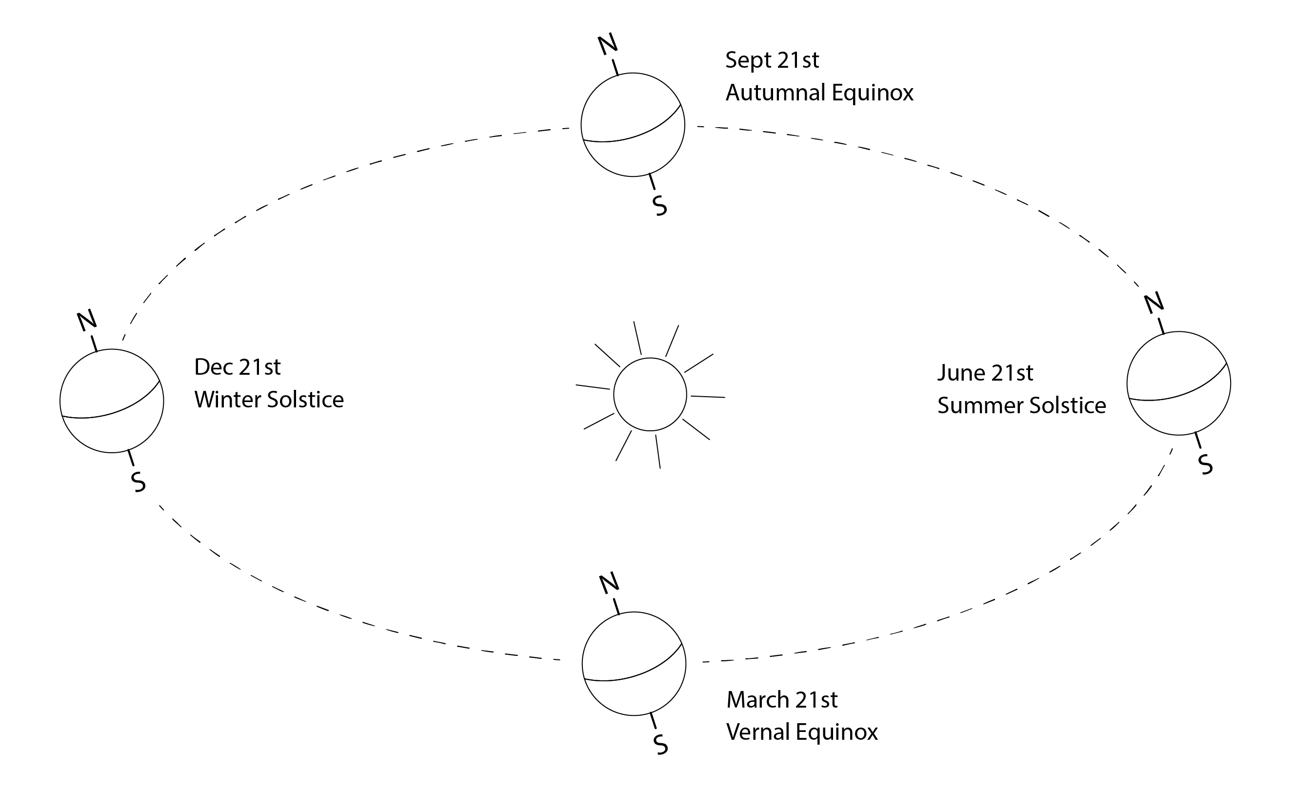
As we know, the Earth orbits the sun every 365.25 days and it takes 24 hours to complete a full rotation. The axis that passes through the North and South poles is also tilted, by approximately 23.45^o. During the summertime, locations with a latitude in the Northern Hemisphere are oriented towards the sun for longer periods than those in the Southern Hemisphere, effectively increasing the solar day length D. Conversely, during the winter months this solar day length is shorter, as our location is oriented away from the sun for longer. This is determined by an angle called the solar declination angle ( $+23.45 \le \delta \le -23.45.$ ). During the spring and autumnal equinoxes, the sun rises above the horizon at a solar time of 6 am and sets 12 hours later.

Figure 1: The Earth’s trajectory around the Sun and the corresponding declination angle

This solar declination angle (in degrees) can be calculated, to a good approximation, as follows: $\delta = 23.45 \sin((360(n+284)/365) \cdot \pi/180)$ , where n corresponds to the Julian day number, so that n = 46 corresponds to the 15th February, and the latter term in brackets ( $\pi/180$ ) converts from degrees to radians for the trigonometric calculation. We can thus simplify this to:

(1) $\begin{equation*} \delta = 23.45 \sin(2 \pi (284+n)/365) \cdot \pi/180 \end{equation*}$

In which the latter term now converts our declination angle from degrees to radians.

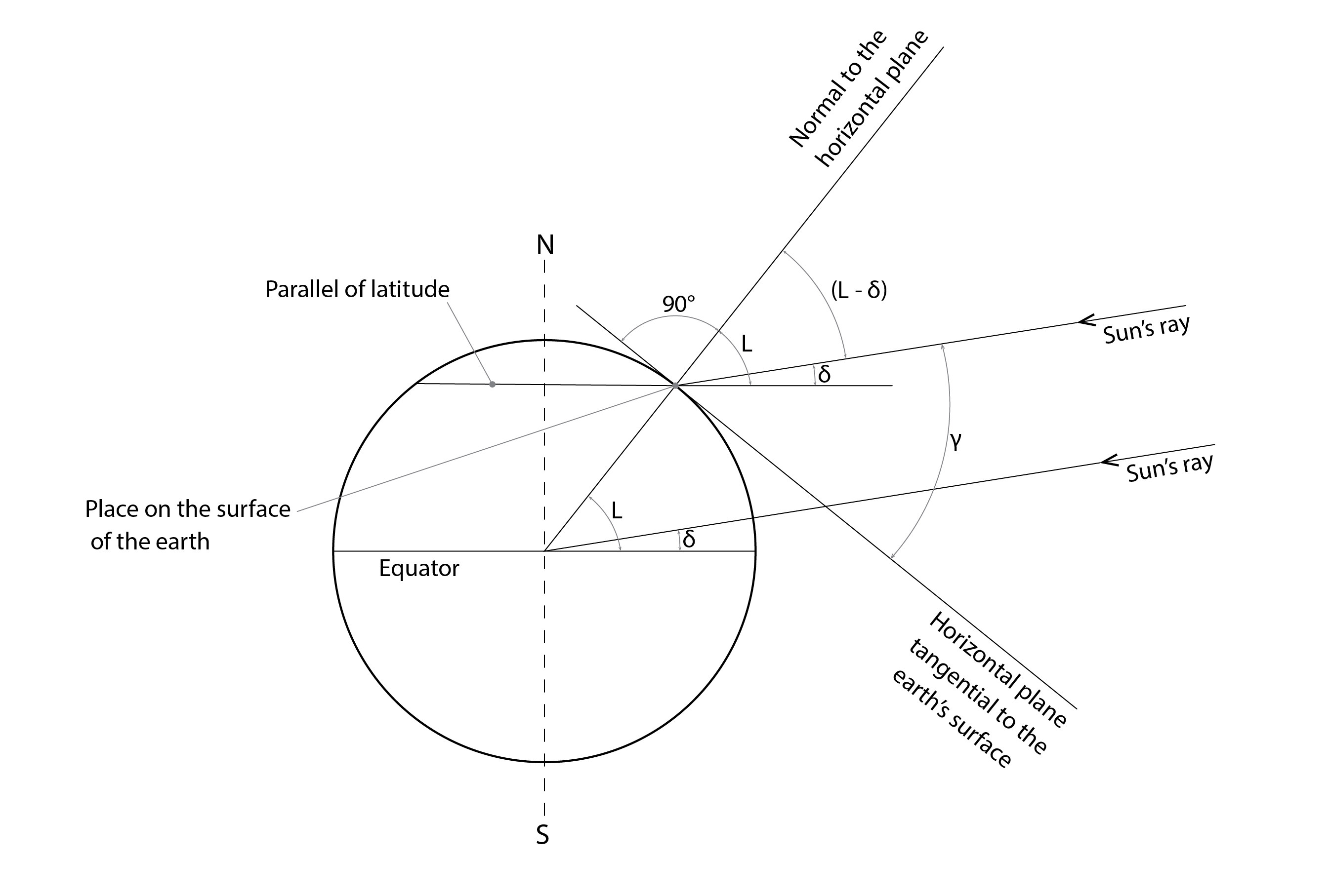
With this and knowing the latitude (l) of our location, we can calculate the solar altitude $\gamma$ in radians:

(2) $\begin{equation*} \gamma = \arcsin(\sin l \sin \delta - \cos l \cos \delta \cos \omega) \end{equation*}$

given the solar hour angle ( $\omega$ ) that corresponds to a particular time ( $t$ ), where $\omega = \pi t/12$ , so that this hour angle spans the range $0 \le \omega \le 2\pi$ . There is an interesting special case, whereby the solar altitude at solar noon is simply: $\pi/2-(l-\delta)$ . For a latitude of 60^o the peak solar altitude (in degrees) at the summer solstice would then simply be $90-(60-23.45) = 53.45^o$ .

Figure 2: The special case of solar altitude at noon

To determine the angular position of the sun, we need to complement our solar altitude with a solar azimuth $\alpha$ or orientation in degrees from North, ^oN:

(3) $\begin{equation*} \alpha = \arccos(-\sin\gamma * \sin\gamma + \sin \delta) / (\cos l * \cos \gamma) \end{equation*}$

(for $\hspace{0.1cm} \omega < \pi$ )

(4) $\begin{equation*} \alpha = 2\pi - \arccos(-\sin\gamma * \sin\gamma + \sin \delta) / (\cos l * \cos \gamma) \end{equation*}$

(for $\omega \ge \pi$ )

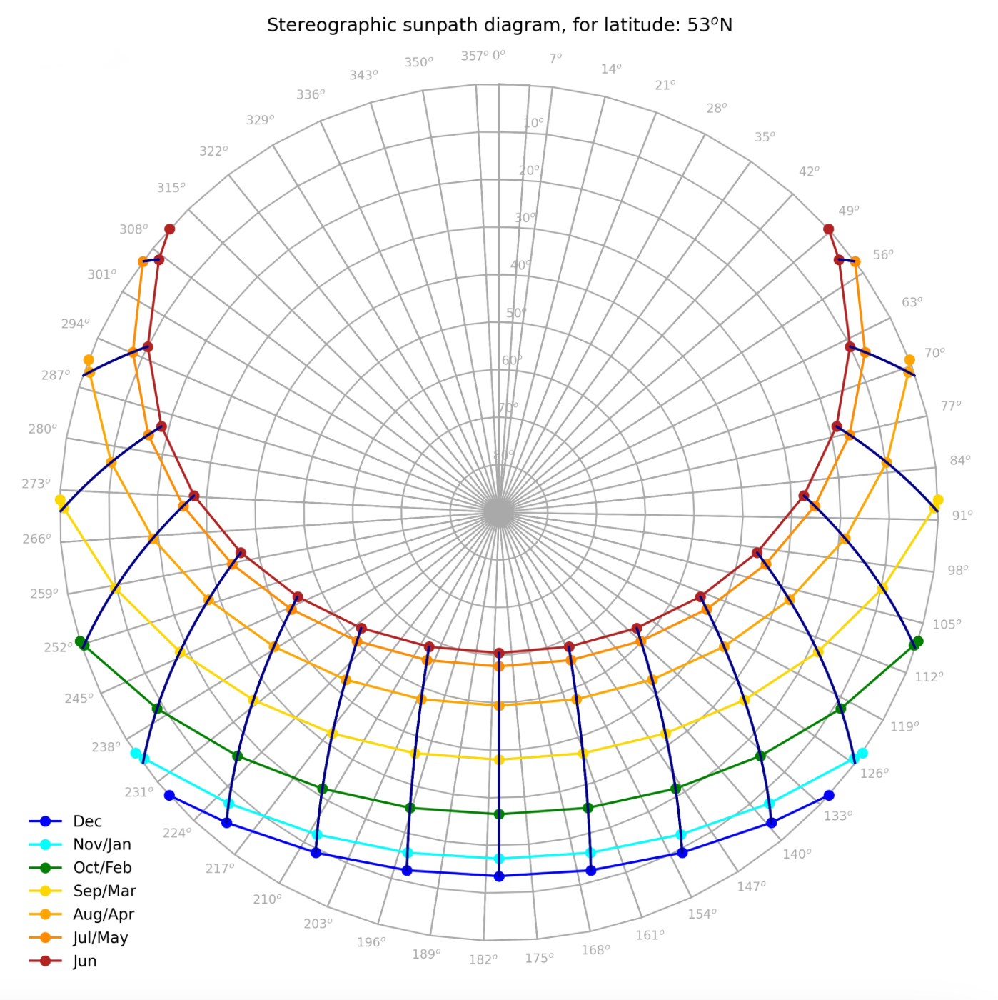
Now that we know how to calculate the solar azimuth and altitude, we can plot a sunpath diagram. The starting point for this is to plot a series of concentric circles representing curves of iso-altitude ( $\gamma_{iso}$ ), as well as a series of spokes of iso-azimuth ( $\alpha_{iso}$ ). If we construct these curves and spokes at 10^o increments, then we simply need to determine the corresponding x,y coordinates, where for example $x_{\gamma} = \gamma_{iso}.\sin \alpha)$ and $y_{\gamma} = \gamma_{iso}.\cos \alpha)$ , where $\alpha$ is expressed in radians. We can then also plot the sunpath lines, from sunrise to sunset on the 21st of each month, from the winter solstice through to the summer solstice, where the sunrise or sunset time is $12\pm L/2$ , where L is the day length: $L=24 \cdot \arccos(-\tan l \tan \delta)/\pi$ . At these times, the altitude is zero ( $\gamma=0$ ), but not (necessarily) the azimuth, and between sunrise and sunset our altitude is above the horizon, so $\gamma >0$ . 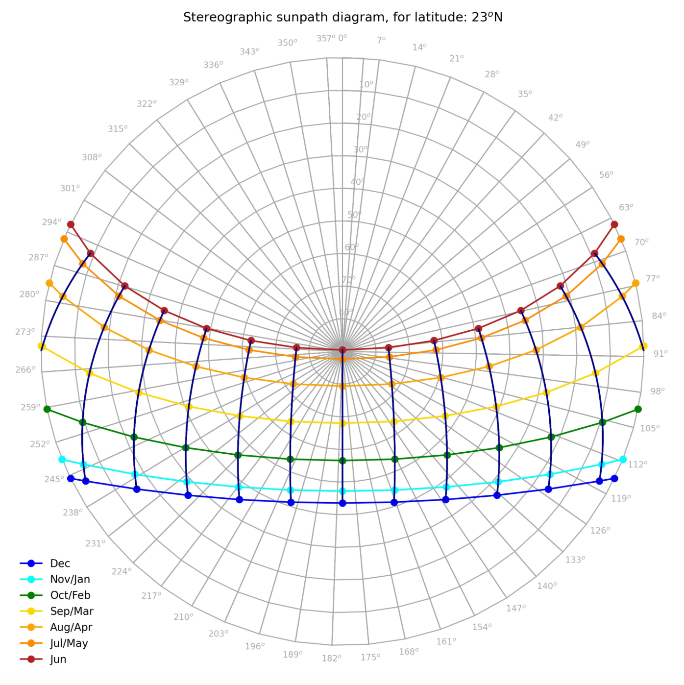The sunpath diagram below ^[1] has been generated for the tropic of Cancer, where $l=\delta_{summer solstice}$ , so that the sun passes about the zenith at noon on the summer solstice.

Figure 3: Sunpath diagram for the Tropic of Cancer

Once we know the solar altitude and azimuth, it is relatively straightforward to calculate the solar irradiance that is incident on a receiving surface, such as a wall, window or a solar (thermal or photovoltaïc) collector. For this, we simply need to multiply the beam irradiance ( $I$ ), the irradiance received on a plane that is normal (or perpendicular) to the sun, as indicated in Fig 4 below, by the cosine of the angle of incidence ( $\cos\theta$ ), so that $I_\theta=I \cos\theta$ .

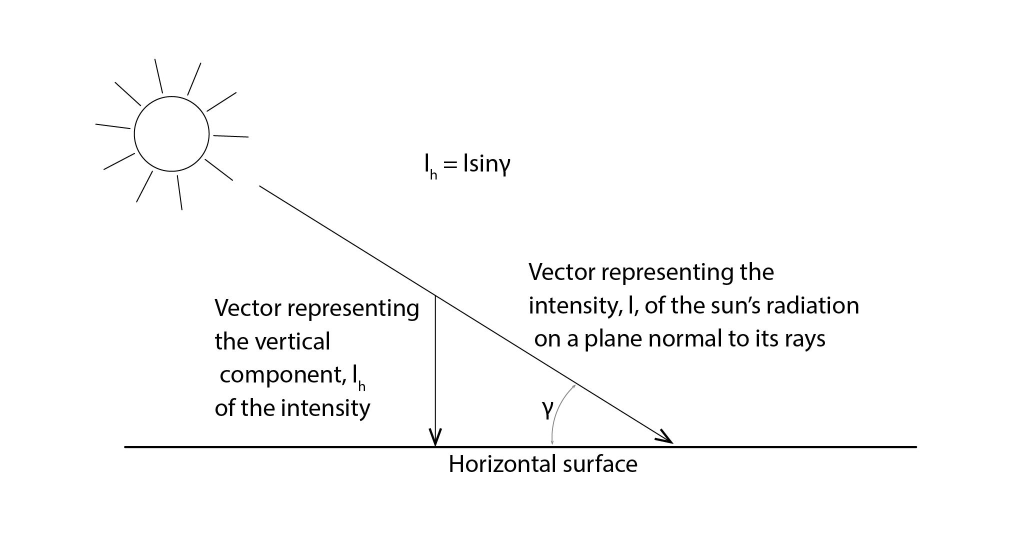
Suppose that we wish to calculate the beam irradiance incident on a flat roof surface. This simply requires that we multiply the beam irradiance that is perpendicular to the position of the sun, call this I, by the sine of the altitude (or the cosine of the zenith angle, $\pi/2-\gamma$ ): $I_\theta = I \sin\gamma$ .

Figure 4: Irradiance incident on a horizontal surface

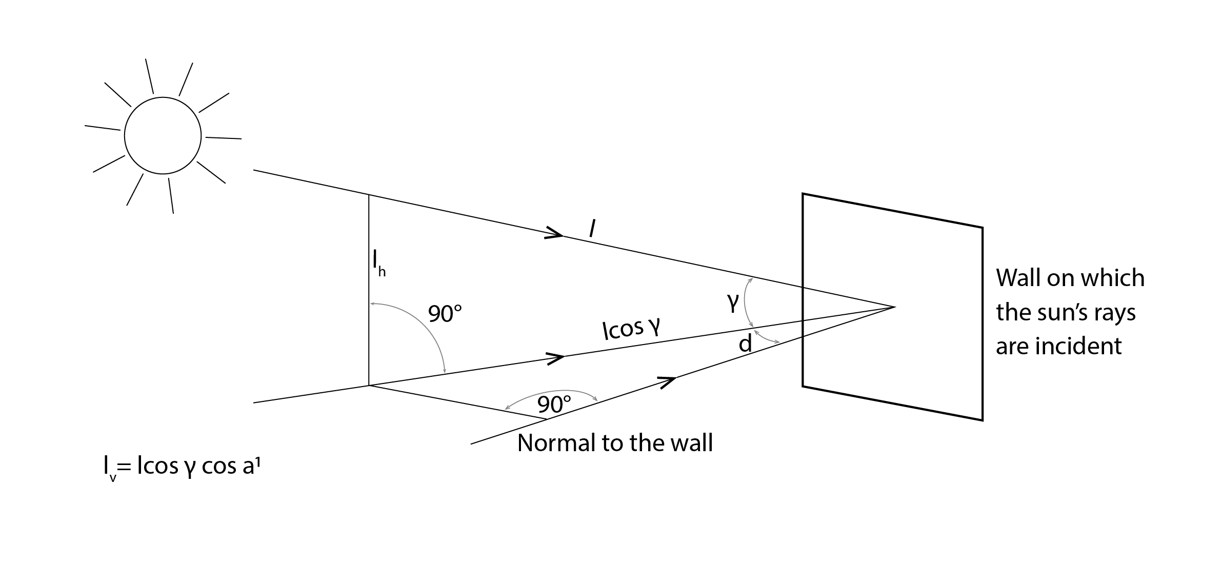
If on the other hand, we wish to calculate the irradiance incident on a vertical surface, we must account for two components: the effect of the sun’s altitude as well as the fact that the sun’s azimuth may not be perpendicular to our receiving surface. For this latter, we calculate a wall-solar azimuth angle, essentially just the difference between the wall’s azimuth and that of the sun ( $\alpha^\prime$ ). So, if our wall has an azimuth of 180^o and the solar azimuth is 210^o then $\alpha^\prime$ = 30^o (or $30\pi/180$ , in radians). Combining these two factors, we can now calculate the beam irradiance incident on our vertical surface:

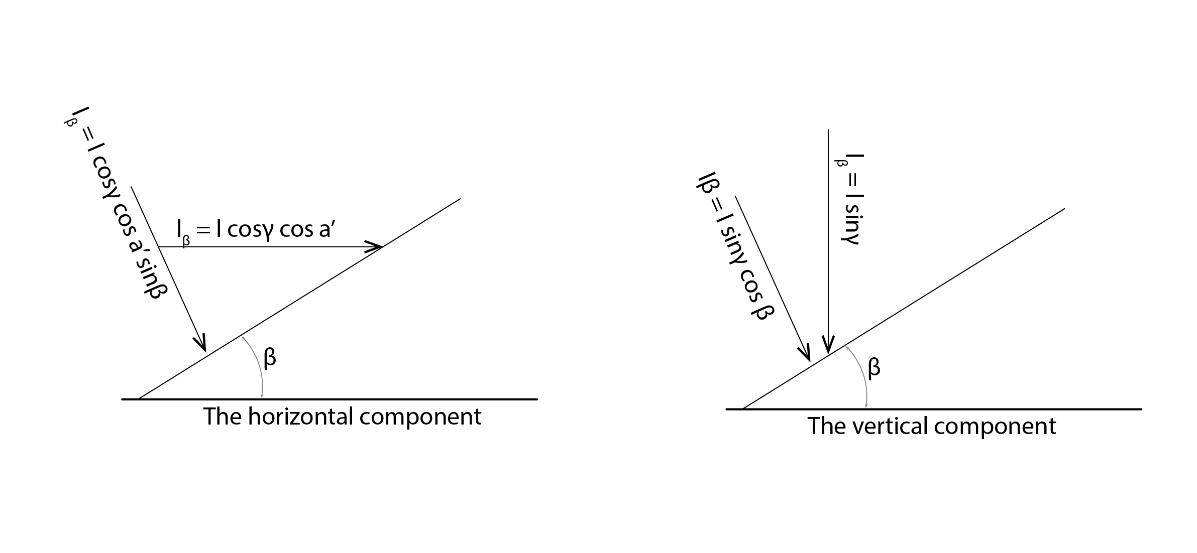
(5) $\begin{equation*} I_\theta=I\cos\gamma \cos\alpha^\prime \end{equation*}$

Figure 5: Irradiance incident on a vertical surface

For the general case of a surface that is tilted at an angle $\beta$ from the horizontal (so that $0\le \beta \le \pi$ ), we now need to multiply our vertical vector by the cosine of this slope and a horizontal vector by the sine of this slope. We can then simply add these two vectors or, more conveniently, we can calculate a combined cosine of the angle of incidence:

(6) $\begin{equation*} cos\theta = \cos\gamma \cos\alpha^\prime \sin\beta + \sin\gamma \cos\beta \end{equation*}$

and the beam irradiance on a surface of any tilt, any orientation and at any location on Earth ( $I_\beta$ ), is simply: $I_\beta=I cos\theta$ .

Figure 6: The general case of irradiance incident on a surface of arbitrary tilt and orientation: considering the joint contribution of horizontal and vertical components.

5.2 Sky radiation

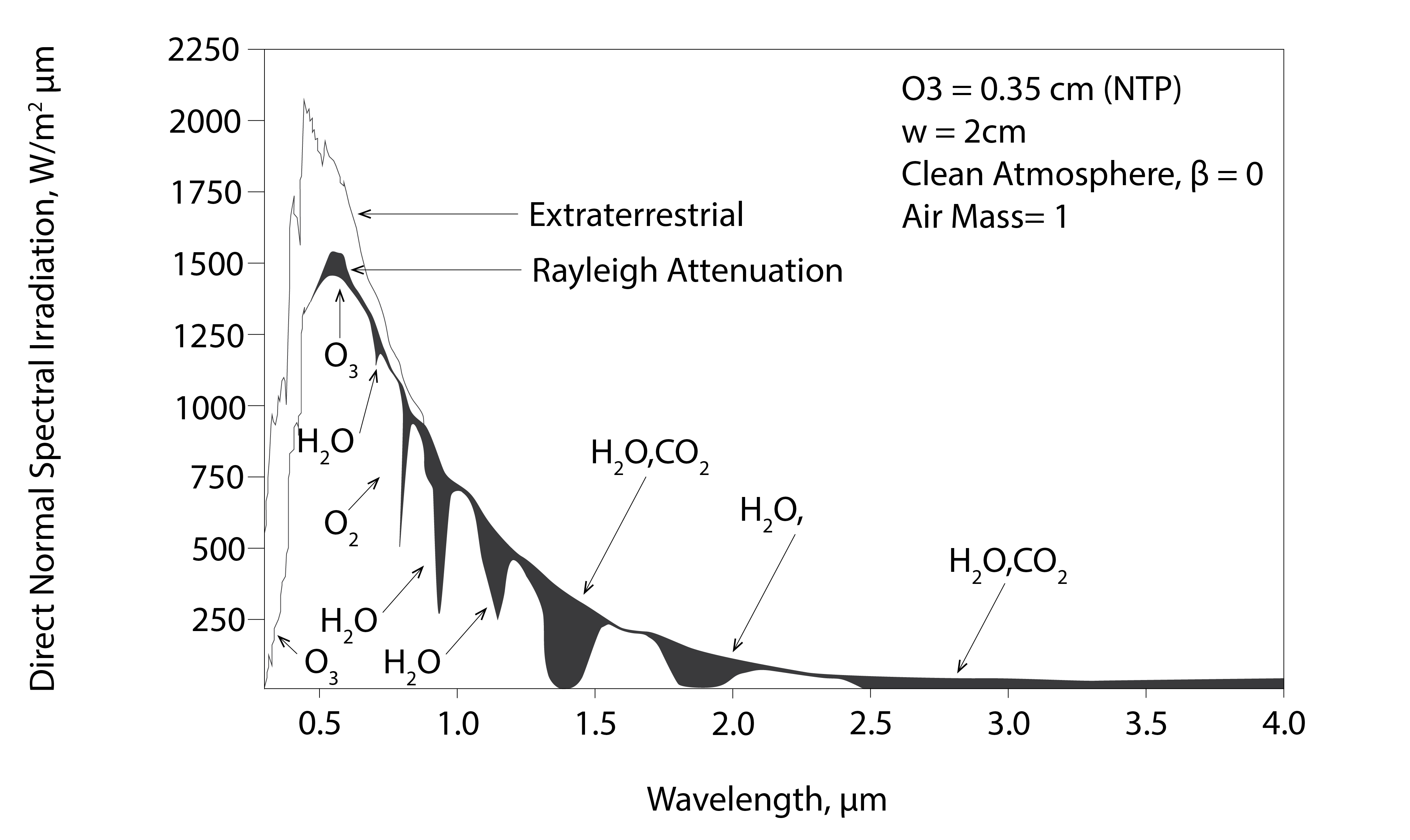
The irradiance incident on the outer atmosphere of the Earth, some 1,367 W/m², is attenuated due to a combination of scattering and absorption. There are two categories of scattering process, referred to as Rayleigh and Mie scattering. Rayleigh scattering is due to interactions with air molecules and varies with $1/\lambda^4$ , so this biases scattering within the blue region of the visible part of the electromagnetic spectrum (the visible part of the spectrum which spans from 380nm to 780nm). This is why clear skies appear blue in colour. Mie scattering is due to interactions with relatively large dust and water molecules (having a diameter greater than the wavelength). Mie scattering is not strongly wavelength dependent, which is why overcast and foggy skies appear white. Finally, some of the incoming solar energy is absorbed by the gases from which the atmosphere is comprised, due to transitions in the magnetic and electric dipole moments of the electrons orbiting the atoms of these gases. Shown in black below are absorption bands corresponding to Oxygen (O₂), Ozone (O₃), Water (H₂O) and Carbon Dioxide (CO₂).

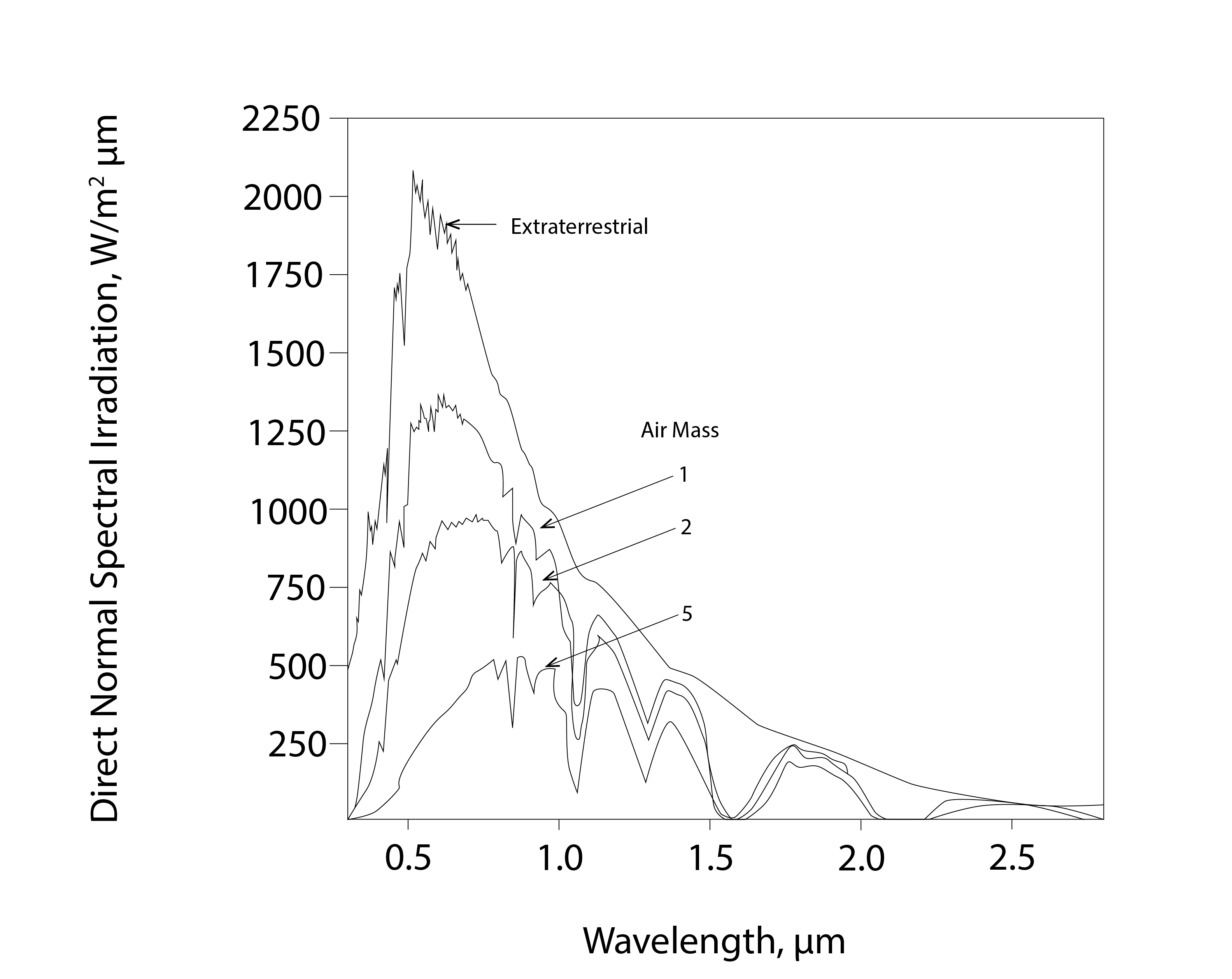
Figure 7: Spectral irradiance distribution (adapted from Duffie and Beckman, 1991)

When solar energy enters the atmosphere at the zenith, it passes through what we refer to as a single unit of air mass. At lower incoming altitudes, this energy passes through multiples of air mass, further attenuating the incoming solar radiation before it reaches the Earth’s surface. In this case, solar energy in the blue part of the spectrum can be fully scattered before reaching the Earth’s surface, giving sunsets (when the solar altitude is low) their red appearance.

Figure 8: Atmospheric attenuation (adapted from Duffie and Beckman, 1991)

5.3 Total solar irradiance incident on a surface

The total solar irradiance incident on a receiving surface ( $I_{Tot}$ ), such as a vertical wall, consists of three components. Earlier, we saw that direct solar irradiance is due to the radiation received directly from the sun ( $I_\beta$ ). In addition to this, our wall receives a contribution of diffuse solar energy from the sky ( $I_{d,sky}$ ) and a further contribution of diffuse solar energy from the ground ( $I_{d,gnd}$ ), so that.

$I_{Tot}=I_\beta + I_{d,sky} + I_{d,gnd}$

Now, one of the most important inputs to a building energy simulation program is a weather file. For example, the software EnergyPlus reads in Energy Plus Weather files (.epw). In addition to metadata describing the latitude, longitude, altitude and the name of the weather station, these files contain hourly weather data. This data mainly relates to six parameters: the beam solar radiation ( $I$ , W/m²), the diffuse sky radiation measured on a horizontal plane ( $I_{sky}$ , W/m²), the air (dry bulb) temperature (^oC), the relative humidity (%) and the wind speed (m/s) and direction (^oN). Sometimes, the beam solar radiation isn’t provided directly, but instead needs to be calculated from the total solar energy measured on a horizontal plane, generally referred to as the global horizontal solar irradiance ( $I_{gh}$ ). From this, we first subtract from the global irradiance, the contribution from the sky, to leave the direct irradiance incident on the horizontal surface, and then divide by the sine of the solar altitude: $I=(I_{gh}-I_{sky})/\sin\gamma$ . It is then relatively straightforward to calculate $I_\beta$ .

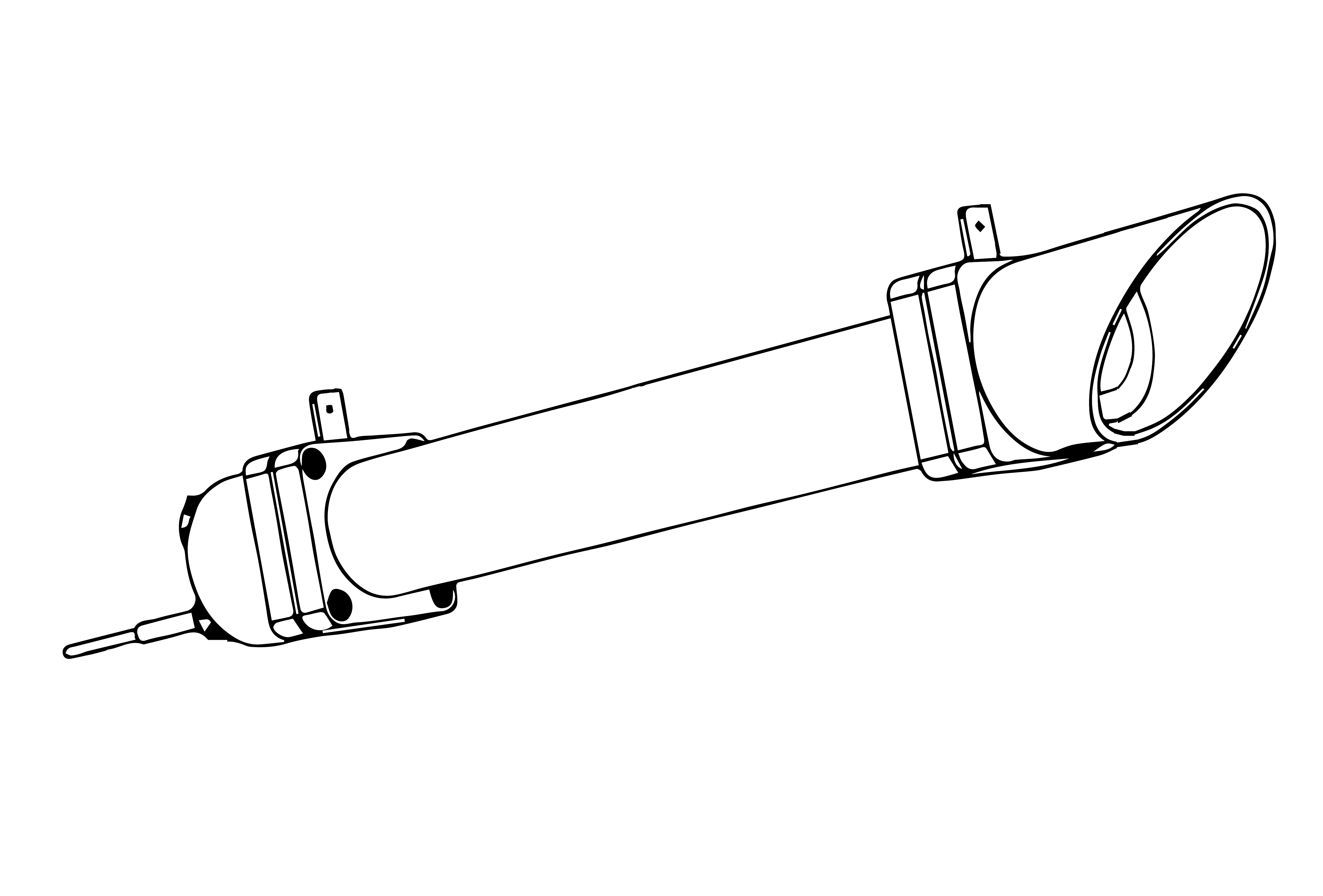
Beam irradiance is measured using a pyroheliometer (shown conceptually in Fig 9 below) that is mounted on a computer-controlled platform to ensure that the inlet to this device is consistently perpendicular to the sun.

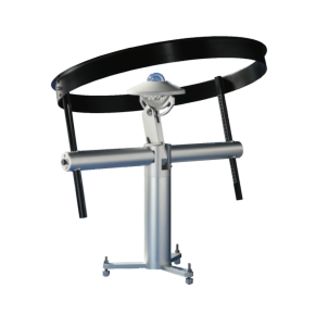
Figure 9: A pyroheliometer for the measurement of beam irradiance

Sky radiation is measured using a shaded band radiometer, where this band is regularly manually adjusted to ensure that the sun is obscured from the radiometer. In the absence of a shaded band, this same device would also measure global horizontal irradiance.

Figure 10: A shaded band radiometer for the measurement of sky radiation

Just as the beam irradiance may be incident on a tilted surface, in the general case, so too may the diffuse irradiance due to the sky and the ground. The simplest situation is if we assume that the sky has the same brightness in all directions; that it is isotopic. In this case, the sky irradiance incident on a tilted surface can be calculated as follows:

$I_{d,sky} = I_{sky}(1+\cos\beta)/2$

so that a horizontal surface would receive all of the available sky radiation and a vertical surface ( $\beta=\pi/2$ ) would receive only half of this amount. In a similar way, we may also calculate the diffuse irradiance that is incident on our tilted surface following reflection from the ground:

$I_{d,gnd} = I_{gh}\rho_{gnd}(1-\cos\beta)/2$

where $\rho_{gnd}$ represents the solar reflectance of the ground, typically assumed to be about 0.2 (though this can vary with the spatial context and also with the season, particularly in cold climates that are prone to snowfall).

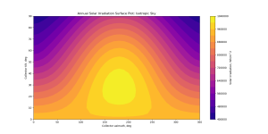
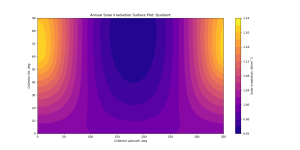
Shown below is a distribution of annual solar irradiation availability from the sun and the sky, calculated assuming that the sky brightness distribution is isotropic.

Figure 11: Total solar irradiation availability for an isotropic sky

Presented below is the same type of image, but now calculated using a relatively sophisticated ^[2] statistical model of the variation of the brightness of the sky as a function of azimuth and altitude throughout the year (see Chapter 2 in Robinson (2011) for further information about this model). Subjectively speaking, this appears to be reasonably similar to that for the above isotropic case.

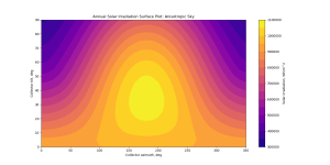
Figure 12: Total solar irradiation availability for an anisotropic sky

However, if we create a new image by dividing the result from the isotropic model by that from the anisotropic model, we observe a considerable deviation. Our isotropic model considerably under-predicts the amount of solar energy that is available in the Southern part of the sky vault (for the location of Sheffield, in the UK) and over-predicts that which is available in the Northern part of the vault.

Figure 13: The quotient of anisotropic and isotropic irradiation distributions

5.4 Shading analysis

Consider a building that is oriented so that its long axis is 20^o East of due South. This is indicated by the black dotted line in the sunpath diagram below. The region of the sunpath diagram that is to the right of this dotted line is behind the wall that interests us: the long wall that has an azimuth of around 290^oN. As such, all of these sun positions are already invisibly to our wall: it is self-shaded from these sun positions. However, all of the sun positions to the left of this line are in principle visible to our wall.

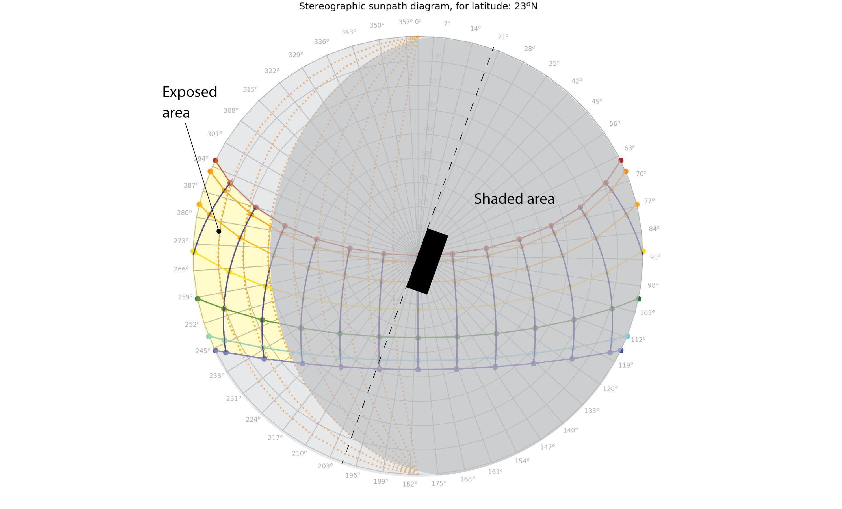
Figure 14: Horizontal shading protractors

However, if we were to add horizontal louvered shading devices to protect the glazing on this wall, with the geometry indicated below (somewhat unrealistic 1m deep projections of louvre that are vertically spaced 0.36m apart from one another) then the worst case scenario would be that at the junction between our glazing and the upper surface of these louvres, we would have a clear line of sight above the horizon of 20^o in altitude when looking perpendicular from this surface^[3]. All regions of the sky above this altitude, represented in grey for the part of the sunpath diagram that is to the left of our dotted axis, are now invisible to our glazing. The louvres protect our window from these sun positions. Our wall is now only exposed to sun positions within the region shaded yellow in the above diagram. This exposed region relates to periods relatively late in the afternoon, from around 4 pm onwards, when the solar altitude is relatively low. If there were buildings opposite this wall, then those buildings would provide additional solar protection within this exposed region.

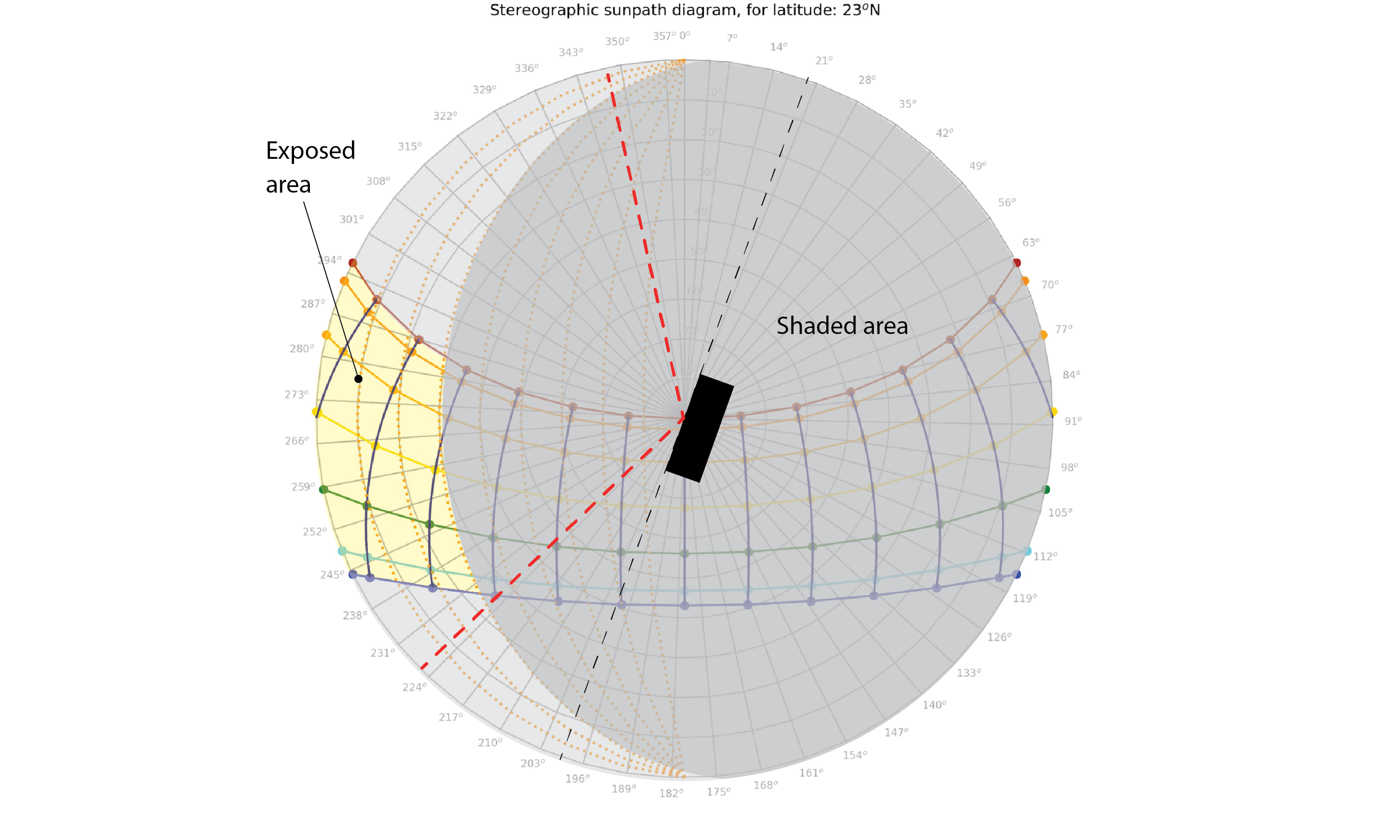
Consider now the addition of vertical fins to our wall. The figure below illustrates a case of shading fins (or vertical louvres) that offer later protection to +/- 30^o from 90^o+/- the azimuth of our wall (taken from the centre point of the glazing).

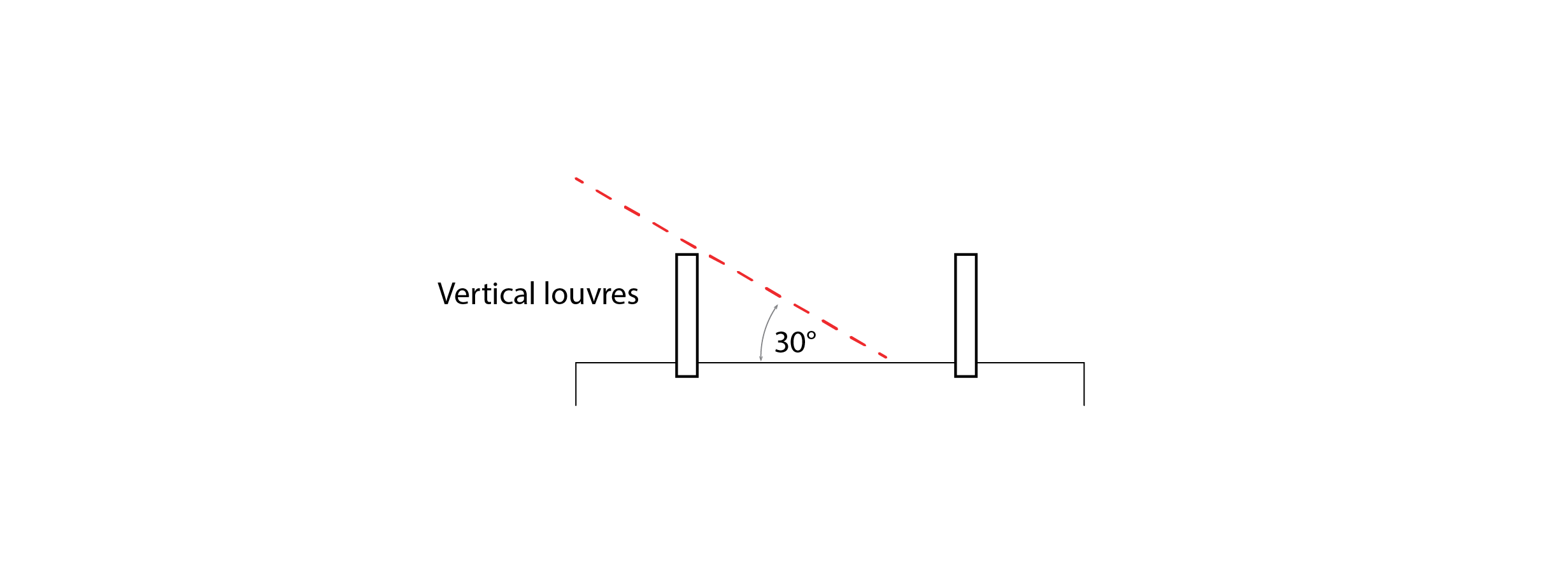
The region between the dotted red lines and the dotted black line in the sunpath diagram below identifies the region of the sky, and thus the corresponding sun positions, for which our wall is protected by these fins. In this case, the right-hand fin provides no useful contribution and the left-hand fin provides less of a contribution than the horizontal louvres do. Furthermore, the protection that these vertical fins offer is biased towards the periods of greatest solar intensity in the wintertime, when the transmission of solar energy would be most useful in displacing the need for applied energy to heat our building. As such, the use of horizontal louvres would appear to be most effective in this case.

Figure 17: The addition of vertical shading

5.5 The difference between clock and solar time

Sunpath diagrams are typically produced to illustrate the position of the sun that corresponds to solar time. The above diagram produced for the Tropic of Cancer identified sun position at hourly intervals from sunrise to sunset for the 21st of each month by solar curves. The solar curve that is due South on the winter solstice (the 21st December) corresponds to solar noon. If we track the sunpath in the Easterly direction for the winter solstice we see that the sun rises a little more than five hourly sun positions before this time, a little earlier than 7 am. Symmetrically, the sun sets shortly after 5 pm in solar time (i.e. 5 hours after rather than before noon).

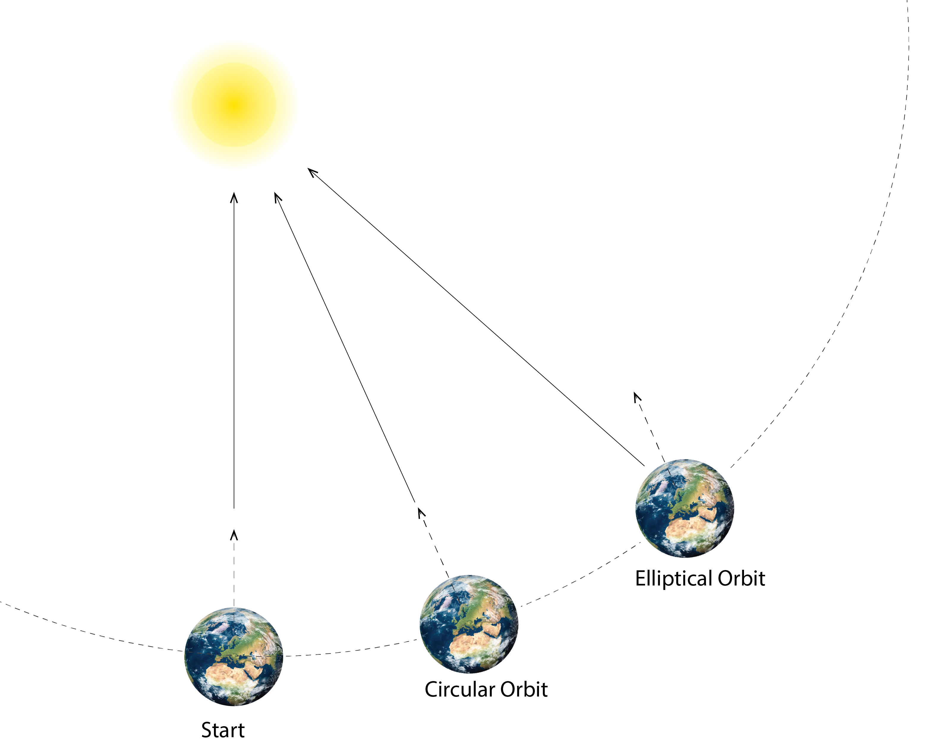
However, the sun is not always oriented due South when the time on a clock or watch reads 12 noon. In fact, the variation of the position of the sun at 12 noon throughout the year appears as a figure of eight – as illustrated in the sunpath diagram below. This is referred to as the analemma and it is caused by two superimposed phenomena: the ellipticity of the Earth’s orbit around the sun and the tilt of the Earth with respect to the sun. The first phenomenon means that, as the Earth orbits the sun, there are occasions when the Earth travels faster (near the long axis of the ellipse). Relative to a circular orbit, this means that the Earth has travelled further, so that the sun appears slightly West of due South at noon, in contrast to a circular orbit where the sun would be due South.

Figure 18: Sunpath diagram in clock time for the latitude of Sheffield, UK

This effect is illustrated in the diagram below (for further information see: https://www.analemma.com/intro.html), in which the virtual Earth B has followed its true elliptical orbit, compared with a fictitious Earth A that has followed a circular orbit.

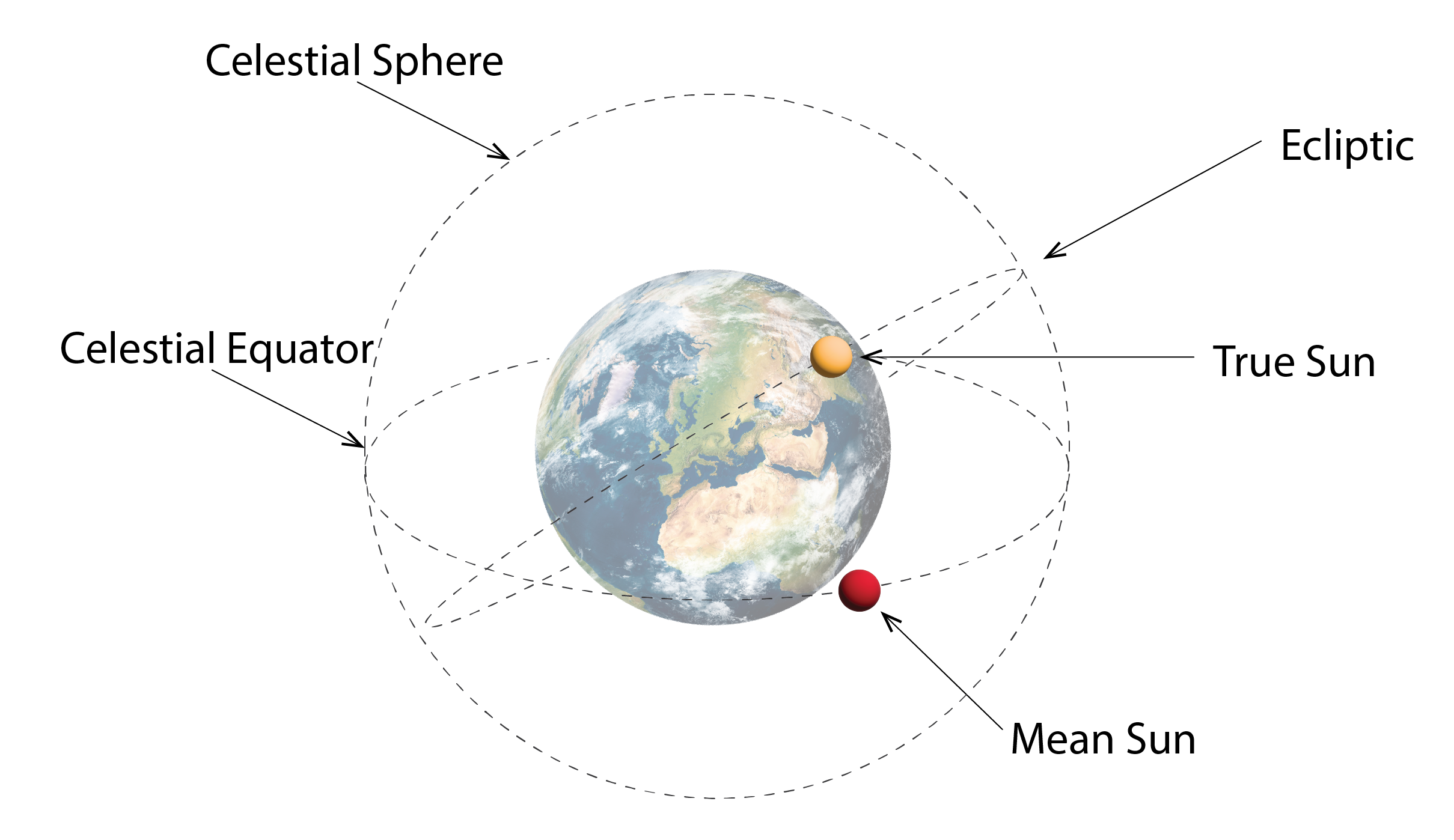
Figure 19: Variation of sun position due to orbital ellipticity

The tilt of the Earth causes a similar effect, so that the plane of the Earth’s rotation about the sun is also elliptical and not circular. The latter is represented by the celestial equator for a hypothetical untilted Earth and the former is represented by the plane of the ecliptic for our true tilted Earth. This means that at noon in clock time, the position of the sun differs between these two cases (for a tilted and an untilted Earth).

Figure 20: The difference in mean sun position (for a virtual untilited Earth) and the True position of the Sun for our tilted Earth

These two effects combine to create a deviation between clock time and solar time, to express the difference in the azimuth of the sun during the course of a year. This is calculated using an equation called the equation of time, and is indicated below.

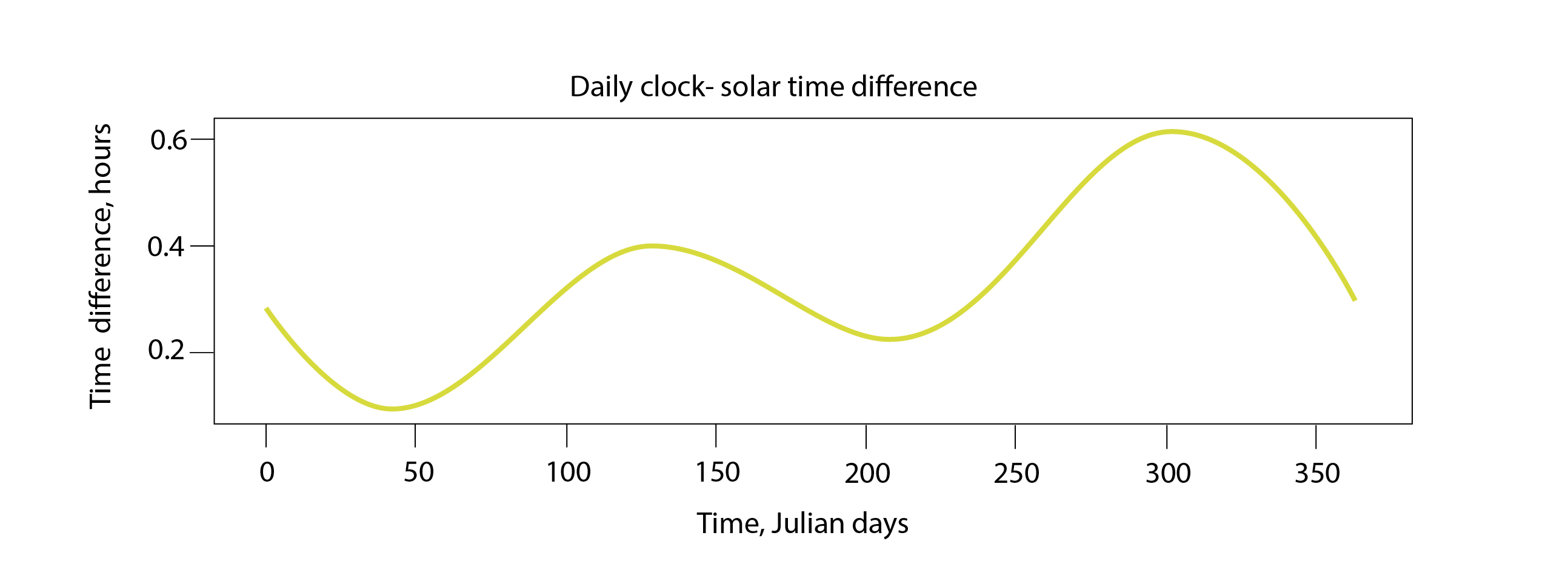
Figure 21: The combination of ellipticity and obliquity, calculated by an equation of time

This, in addition to daylight savings time, can impact the usefulness of solar shading devices during the periods in which a building (in particular a workplace) is occupied.

5.6 Questions and worked examples

This section contains a series of worked examples or problems (P) and their solutions (S), as well as a series of written questions (Q) and their written answers (A).

P1) Calculate the solar declination angle for the 21st of June.

P2) For a latitude of 52 degrees, calculate the sunrise time for the day in P1.

P3) Calculate the solar altitude and the solar azimuth at 11 am on this day.

P4) Now, calculate the cosine of the angle of incidence ( $\cos \theta$ ) using these solar coordinates, on a vertical south-facing surface.

P5) Repeat this calculation sequence for the 21st December, Julian day number 355.

S1) First we need to determine that the Julian day number for the 21st of June is 172. Entering this into our declination angle equation, we see that the corresponding declination angle is 0.407 rads (or 23.45^o) as we would expect.

S2) The day length for this day at this latitude is 16.5h, so the sunrise time is 03:45 am.

S3) We first of all need to calculate the hour angle. At this hour we have that $\omega$ has a value of 2.88 rads. With our previous declination angle and our latitude, the solar altitude using this hour angle is 1.03rads (or 59^o) and our solar azimuth, using this altitude, is 2.66rads (or 152^o).

S4) Using the equation for $\cos \theta$ presented earlier, our cosine of the angle of incidence is 0.45.

S5) The value for $\cos \theta$ for the winter solstice is now 0.94.

Q1) If the beam irradiance is 400W/m² and 750W/m² at the winter and summer solstices respectively for the surface at the tilt, azimuth and location studied in the above problems, which would be more effective at converting solar irradiance into heat, either to heat hot water or to heat the interior space of a room?

A1) Although the winter beam irradiance is lower, the cosine of the angle of incidence is far higher. The incident beam irradiance is 377Wm² compared to 340W/m² in the Summer case. Our surface would clearly be more effective at supporting solar heating in winter than in summer.

References

Duffie, J.A., Beckman, W.A. (1991), Solar Engineering of Solar Processes. Wiley – Interscience, 2nd Ed, 1991.

Robinson, D (2011), Computer modelling for sustainable urban design, Taylor and Francis, 2011.

Note that this Sunpath diagram has been produced using my PyClim Web App (which can be accessed from the link here). Similar diagrams can be produced using this app for any location on Earth. ) ↵
Although considerably more complex models of anisotropic sky brightness distribution do exist. ↵
Note that, for deviations from the perpendicular, this apparent altitude $\gamma^\prime$ is lower. The altitudes of the orange curves in the above sunpath diagram that correspond to horizontal shading protractors are calculated thus: $\gamma^\prime = \arctan(\tan\gamma \cos \lvert \alpha_w - \alpha \rvert)$ , where $\alpha$ refers to the azimuth of either our wall $w$ or of a deviation from this perpendicular for one of our louvres ↵