Psychrometry, condensation and enthalpy

Darren Robinson

2 Psychrometry, condensation and enthalpy

This chapter introduces the fundamental principles concerning the psychrometric (see s2.1 below) state of humid air, the circumstances under which moisture will condense out of this air and how to calculate the work that is done to condition air to meet a room’s demand for heating and cooling, to maintain occupants’ comfort requirements, as well as for the provision of fresh air to these occupants.

2.1 Psychrometry

Derived from the Greek ψυχρόν (psuchron) for cold, and μέτρον (metron) for means of measurement; psychrometry is concerned with the physical and thermodynamic properties of gas-vapour mixtures. According to the ideal gas law:

(1) $\begin{equation*} pV=nRT \end{equation*}$

for a gas of temperature T ( $K$ ), contained at a pressure p ( $N/m^2$ ) in a volume V ( $m^3$ ) and comprised of a number n of mols (determined from the mass of a substance m (kg) and its molar mass M ( $kg/mol$ ): $n=m/M$ ), where R is the universal gas constant ( $8.317 J/(mol \cdot K)$ ). From this expression, we can also determine the density of a gas, $\rho$ ( $kg/m^3$ ):

(2) $\begin{equation*} \rho = \frac{m}{V} = \frac{pM}{RT} \end{equation*}$

The moisture content $g$ of air is conventionally measured in kg(water) per kg (dry air): $m_w/m_a$ . Thus:

(3) $\begin{equation*} g=\frac{p_wVM_w}{RT}\cdot\frac {RT}{p_aVM_a}=\frac{p_wM_w}{p_aM_a} \end{equation*}$

The standard molar masses M for water and air are 0.018016 and 0.02861 respectively; the ratio of these two being 0.62197. Thus, the moisture content $g=0.62197p_w/p_a$ . Psychrometric calculations normally take place at a standard atmospheric pressure $p_{at}$ of 101325 (Pa). Knowing, from Dalton’s law of partial pressures, that $p_{at}=p_a+p_w$ , we can also express moisture content as follows:

(4) $\begin{equation*} g=\frac{0.62197p_w}{p_{at}-p_w} \end{equation*}$

The relative humidity of air $\phi$ ^[1] is obtained from the ratio of the partial pressure of water vapour $p_w$ and the partial pressure of saturated water vapour, at the same temperature $p_s$ , so that:

(5) $\begin{equation*} \phi=100p_w/p_s \end{equation*}$

Where this latter ( $p_s$ ) depends exclusively on the dry bulb air temperature t: (Jones, 1994):

(6) $\begin{equation*} \log_{10}p_s = 30.59091-8.2\log(t+0.01)+0.00248 (t+0.01)-\frac{3142.3}{(t+0.01)} \end{equation*}$

(for $\hspace{0.1cm} t\ge 273.15K$ )

and:

(7) $\begin{equation*} \log_{10}p_s = 9.5381 - \frac{2663.9}{(t)} \end{equation*}$

(for $\hspace{0.1cm} t < 273.15K$ ).

The increment 0.01K above expresses the temperature relative to the triple point of water^[2]. From our earlier expression for moisture content $g$ , we can now also isolate the partial pressure of water vapour:

(8) $\begin{equation*} p_w=\frac{p_{at}g}{0.62197+g} \end{equation*}$

Therefore, if we know the values for t and g we can calculate $\phi$ , and similarly, if we know the values of t and $\phi$ we can also calculate g (first calculating $p_w = \phi p_s/100$ and then g from the final corresponding expression above. Thus, with two psychrometric quantities, all others may be deduced.

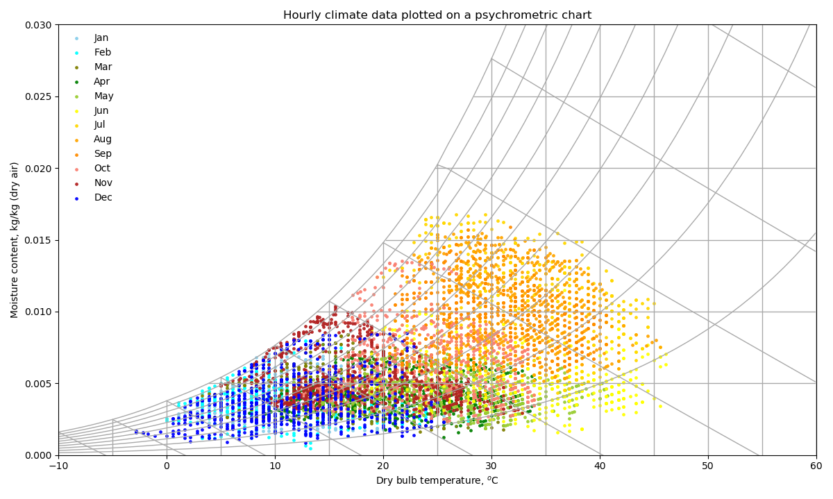
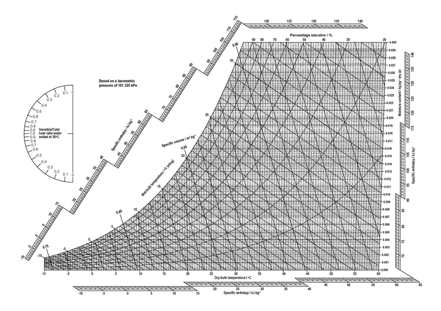
These psychrometric properties form the basis of the psychrometric chart below (Figure 1), in which the curves correspond to relative humidity (or percentage saturation), the horizontal lines correspond to moisture content and the vertical lines correspond to air (dry bulb) temperature. The sloped lines correspond to a quantity called the wet bulb temperature (which is a little trickier to calculate than the other quantities). This is the temperature that would be recorded by a thermometer where the mercury bulb at its base is covered in a wetted gauze, and the bulb is continuously whirled around in a circle until the air around the bulb becomes saturated. Much of the latent heat of vapourisation for this evaporation of moisture is provided by the bulb, lowering the temperature that is recorded by the Mercury until it reaches a steady state. This is the wet bulb temperature.

The coloured circles in our psychrometric chart correspond to hourly conditions of the psychrometric state of air, for a weather file created from data measured in Phoenix, Arizona (US).

Figure 1: Psychrometric chart displaying hourly coincident air temperature and moisture content for Phoenix, Arizona (US)

2.2 Condensation

This section describes the phenomena that lead to moisture condensing out of air onto the surface of a material (surface condensation) as well as that condensing out of air within a material or an assembly of materials (interstitial condensation).

Surface condensation

Take any psychrometric state represented by a coloured circle in the above chart. If we were to cool the air from this initial starting state until it reached the saturation curve (the leftmost curve, which corresponds to a relative humidity of 100%), this air would then have reached its dew point temperature at which the air is completely saturated. This dew point temperature $t_d$ (K) is the temperature at which the partial pressure of water vapour mixed with dry air $p_w$ becomes a saturated vapour pressure $p_s$ . This can be found by using an iterative procedure, adjusting the temperature used in the above equations (6, 7) to calculate $p_s$ until the incremental temperature change is small enough (e.g. two decimal places) that the pressure difference between $p_w$ and $p_s$ are acceptably small (and ensuring that $p_w \ge p_s$ ). Any further cooling of the air beyond this point would cause moisture to condense out of the air. If it was due to contact between our air and a cooler surface $t_{sur}$ , say an internal pane of glass, that caused the air to reach its dew point temperature, then moisture would be deposited on this surface. In other words, surface condensation would occur whilst $t_{sur} \le t_d$ ).

We saw from the previous chapter on “Heat, temperature and thermal energy” that the internal film resistance $R_{si}$ has a value of approximately 0.123 $m^2 \cdot K / W$ . We also saw that the specific heat capacity $C_p$ of air has a typical value of 1000 $J/kg \cdot K$ or 1 $J/g \cdot K$ . From these observations we can calculate the approximate mass flow rate of air in contact with our surface $\dot m_a$ in $g_{air}/(m^2 \cdot s)$ :

(9) $\begin{equation*} \dot m_a \approx R_{si}/C_p \end{equation*}$

which takes a value of around 8 $g_{air}/(m^2 \cdot s)$ . Since we know that there are 1000g of air for each kg of air and that there are 3600s in each hour, we can write that:

(10) $\begin{equation*} \dot m_w \approx \dot m_a(g - g_s) \end{equation*}$

where our units are $[\frac{g_a}{m^2 \cdot s}] \cdot [\frac{g_w}{kg_w}] \cdot [\frac{3600s/h}{1000g_a/kg_a}]$ = $[\frac{g_w}{m^2 \cdot h}]$ , so that the rate at which moisture condenses onto our surface is (while $g \ge g_s$ ):

(11) $\begin{equation*} \dot m_w \approx 28.8 (g - g_s) [\frac{g_w}{m^2 \cdot h}] \end{equation*}$

For this, we need to calculate the moisture content of our internal air ( $g$ [g/kg]). This we can assume is equal to the outside moisture content ( $g_o$ ) [g/kg] plus an internal rate of production of moisture ( $\dot g$ ) [g/h] diluted by the rate at which the internal mass of air is exchanged with the outside $\dot m_a = \rho \cdot \dot V$ [kg/m³ $\cdot$ m³/h]:

(12) $\begin{equation*} g=g_o + \frac{\dot g}{\rho \dot V} \end{equation*}$

Interstitial condensation

Some materials, such as glass, are impervious to the transmission of moisture. However, these are relatively exceptional. Other materials, such as bricks, concrete, timber, plaster and also insulation materials are pervious. In other words, they allow for the transmission of water vapour through them.

To calculate the occurrence of condensation within a material, it is recommended to use the method described in the international standard ISO 13788:2012 (ISO, 2012), normally referred to as the Glaser Method.

Now, we saw in the previous chapter on “Heat, Temperature and Thermal Energy” that the rate of heat flow through the fabric of a wall [W] is calculated using an equation of the form $Q = UA \Delta T = A \Delta T/ \Sigma R$ , where the total thermal resistance of the wall $\Sigma R$ is the reciprocal of the U-Value. Analogously, we can also calculate the rate of water vapour transfer through fabric of a wall ( $Q_v$ [ $kg/s$ ]), using an expression of the form:

(13) $\begin{equation*} Q_v = A \Delta p / \Sigma R_v \end{equation*}$

where $\Delta p$ refers to the total vapour pressure difference across the wall and $\Sigma R_v$ to the total resistance to vapour transmission [ $s \cdot m^2 \cdot Pa/kg$ ], where for each layer of a multilayer construction, $R_v= \frac {l}{k_v}$ . This is entirely analogous to thermal resistance, where k_vrepresents vapour conductivity [ $kg/s \cdot m \cdot Pa$ ].

To quantify the amount of condensation that will occur in our wall, for each month of the year, we need to know where condensation is likely to occur, by plotting the saturation vapour pressure p_s against the vapour pressure p_v between the exterior and interior surfaces. Where the two coincide (for $p_v \ngtr p_s$ ) condensation occurs. The rate of inflow of moisture to these regions less the rate of outflow from them corresponds to the accumulation of moisture ( $Q_{v,in} \ge Q_{v,out}$ ) or indeed the evaporation of moisture ( $Q_{v,in} \le Q_{v,out}$ ).

Worked example

The simplest way of explaining how to determine whether and by how much interstitial condensation is likely to occur in a construction material is by example. Here then, we examine a multilayer wall assembly that is given as an example in the ISO standard mentioned above. The properties of this wall are given in Table 1 below:

Table 1: Material hygrothermal properties
Layer	Thickness, $x$ , m	Thermal resistance, m².K/W	Water vapour diffusion resistance factor, $\mu$ , –	Equivalent air layer thickness for vapour diffusion, S, m
External film		0.05
Render	0.012	0.015	8	0.096
Blockwork	0.275	2.500	10	2.750
Insulation	0.020	0.500	1	0.020
Plasterboard	0.0123	0.023	8	0.104
Internal film		0.123

The expression for Q_v above is akin to Fourier’s law, but now for the diffusion of water vapour, so that $Q_v = -\lambda \delta p /{\delta x}$ [kg/m².s]. Here lambda is the water vapour diffusion in air [kg/(m.s.Pa)]: $\lambda = 2\cdot10^{-7}T^{0.81}/P_{at}$ , where T is the absolute air temperature (K). But construction materials do of course pose a resistance to the diffusion of vapour, $\mu$ . Thus our expression becomes $Q_v = -\ \frac{\lambda}{\mu} \frac{\delta p}{\delta x}$ . The ISO standard suggests multiplying the material thickness by its corresponding resistance factor (column 4 in the above table), to create an equivalent air layer thickness, $S=x \cdot \mu$ ; the final column in the above table, so that $Q_v = -\lambda \frac{\delta p}{\delta x \cdot \mu}$ .

Now, the ISO standard recommends splitting materials that have a thermal resistance greater than 0.25 m²K/W into multiple parts, each having a resistance of 0.25 or lower. As such, our insulation layer becomes two layers and our blockwork layer becomes 10 thinner layers. This is so that the temperature distribution can be better resolved, to determine where condensation is likely to take place (the locations where the material’s temperature drops to or below the dew point temperature ( $t_w \le t_{dpt}$ ), or where the calculated water vapour pressure exceeds the saturation pressure: $p_v \ge p_s$ ). We will determine where and the extent to which condensation occurs in our wall for January, whereby $T_{ao}=-10^oC, T_{ai} = 20^oC, \phi_o=95\%$ , and $\phi_i=49\%$ .

In the example given above, this leads to a temperature distribution (where $t=t_{ai} - R_c \Delta T / U$ and $R_c$ is a cumulative thermal resistance, from the inside towards the outside) that looks as follows (Figure 2):

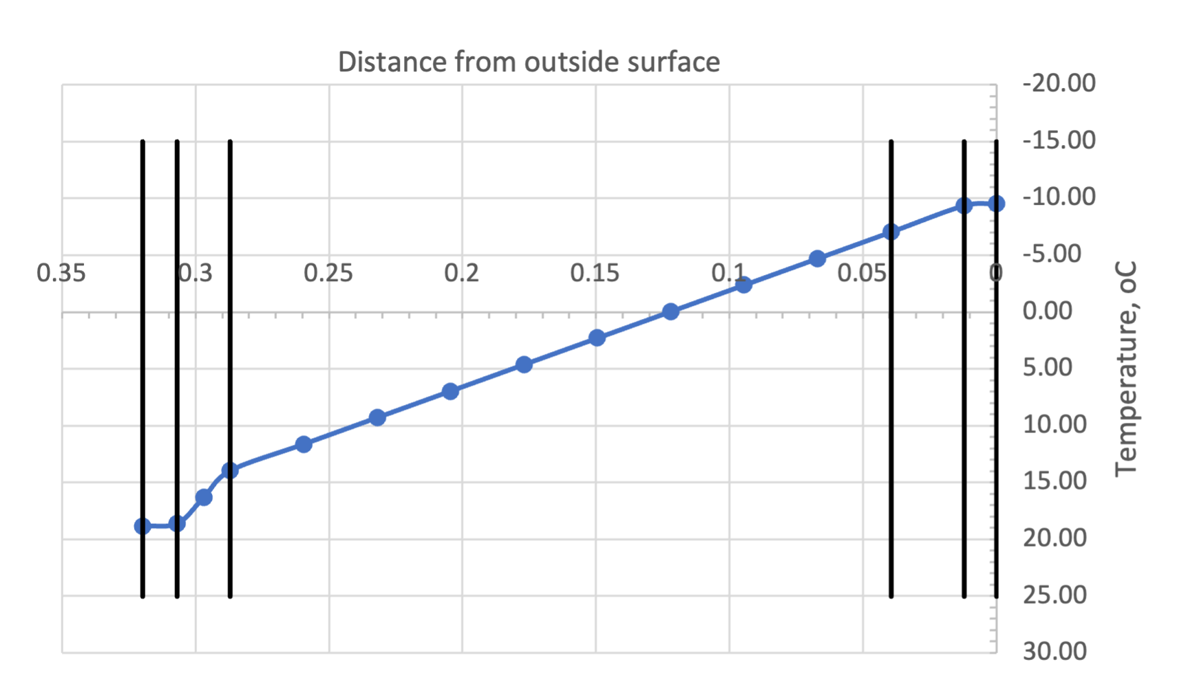
Note that the vertical black lines in Figure 2 correspond to the physical interfaces and the circles in the temperature distribution curve represent both physical and virtual interfaces.

Now that we have our temperature distribution, we can also calculate our saturation vapour pressure $p_s$ for each of the (physical or virtual) interfaces of our wall assembly. We can also calculate the interior and exterior water vapour pressures $p_v$ , assuming the gradient of this from outside to inside to be linear. This gives us the following pressure distributions (Figure 3):

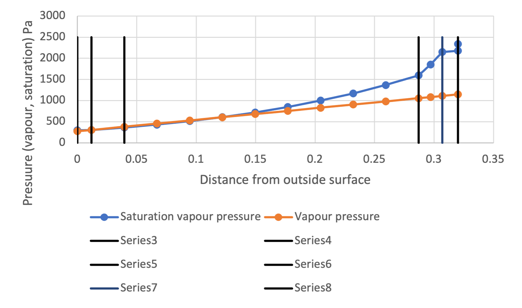
Figure 3: Vapour pressure distribution through the wall

From this (where once again physical interfaces are represented by black vertical lines) we can see that the two curves meet quite close to the exterior surface, at the third virtual interface of the blockwork and that this persists until the outside surface of the render.

Shown below (Figure 4) is an equivalent vapour pressure distribution chart, but now with respect to the vapour diffusion thickness, S.

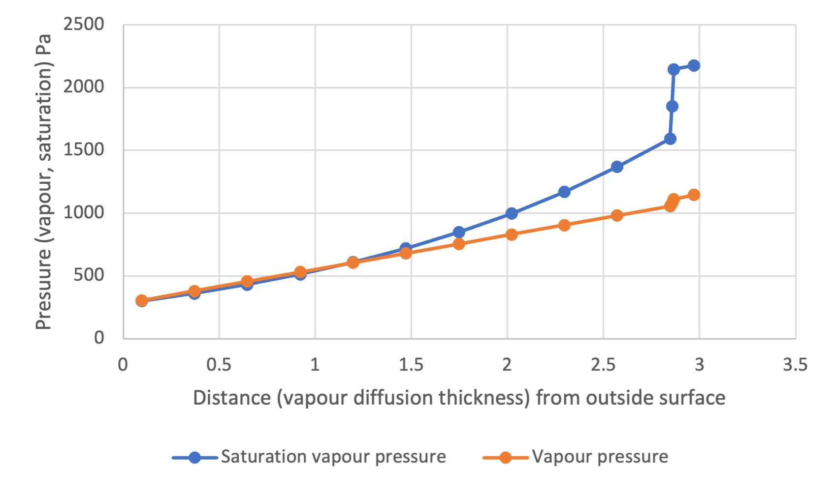
Figure 4: Wall vapour pressure distribution as a function of effective air layer thickness

The rate at which vapour condenses is determined by the rate at which vapour flows into our first interface ( $Q_{v,in}$ ) from the interior less the rate at which it flows out from this region of condensation to the exterior ( $Q_{v,out}$ )^[3]. Our moisture inflow rate $Q_{v,in} = -\lambda \frac{\delta p}{\delta x \cdot \mu}$ , where our pressure difference is determined from the internal water vapour pressure to the saturation vapour pressure at the first condensation interface, call this x: $\delta p = p_{v,i} - p_{s,x}$ and $\delta x \cdot \mu$ corresponds to the total equivalent air layer thickness for vapour diffusion from the inside surface to this point. Similarly, the rate of outflow $Q_{v,out}$ is determined from the saturation vapour pressure at the outer limit of our region of condensation less the water vapour pressure of the exterior $\delta p = p_{s,x} - p_{v,o}$ and $\delta x \cdot \mu$ corresponds to the total equivalent air layer thickness for vapour diffusion from this point to the outside^[4].

Finally we can calculate the amount of condensed moisture that accumulates during a month, call this G [kg/m²], assuming our internal and external conditions to be invariant during this period, as follows: $G=(Q_{in}-Q_{out})\Sigma t$ , where $\Sigma t$ is the total time that has accumulated [s] during this period (2,678,400s for January).

For our case, we have a total accumulation of condensed moisture within our wall of 0.07kg/m².

The ISO standard describes how this calculation procedure can be repeated for different months throughout the year, also explaining how the evaporation of moisture from regions that have accumulated condensation during cooler periods can be calculated. Thus, we can determine whether a wall is able to fully dry out and how long this drying out will take.

2.3 Enthalpy and air-conditioning

Shown below (Figure 5) is the CIBSE Psychrometric Chart; essentially a more elaborate version of the chart that was presented earlier to illustrate climate data for Phoenix, Arizona. As before, the horizontal lines correspond to moisture content, in units of kg moisture / kg of dry air. The vertical lines once again correspond to dry bulb air temperature. The Sloped lines represent the wet bulb temperature. What is unique and different in this chart compared with the previous one, is that at its extremity we have a new quantity, called the specific enthalpy h [kJ/kg] – the enthalpy of the air H (kJ) per unit of mass m (kg) of air – where the enthalpy represents the total internal energy of air (U) and the product of its pressure (p) and volume (V): ( $H=U+pV$ ). If we know what the enthalpy of a particular psychrometric state of air is, then we can determine how much work is required to change that state (e.g. to a cooler or a drier state), for a defined mass flow rate of air. Thus, enthalpy is central to the design and sizing of air-conditioning systems and in determining the demands for energy arising from the use of these systems.

We can calculate the enthalpy of air as the sum of its dry air (h_a) and of water vapour (h_g) component parts: $h=h_a+g \cdot h_g$ , where g is the moisture content of the air.

(14) $\begin{equation*} h_a=1.007(t-273.15)-0.026, \; [273.15 \le t \le 333.15] \end{equation*}$

(15) $\begin{equation*} h_a=1.005(t-273.15), \; [263.15 \le t < 273.15] \end{equation*}$

and:

(16) $\begin{equation*} h_g=2501+1.84(t-273.15) \end{equation*}$

Combining these contributions then, the total specific enthalpy of air above the freezing point of water is:

(17) $\begin{equation*} h=1.007(t-273.15)-0.026 + g(2501+1.84(t-273.15)) \end{equation*}$

where t is the absolute temperature [K].

Thus, any change in the air temperature or the moisture content of air changes its total internal thermal energy. To effect this change, usually implies that work needs to be performed to achieve this change in internal energy.

Consider outdoor air at a state determined by a relative humidity of 50% and an air temperature of around 30^oC, point A in the chart below (Figure 6). The air in this state has an enthalpy of around 65 kJ/kg of air. Suppose that we have an office room that has a floor area of 25m²and is occupied by 5 people, each needing 10 l/s of fresh air, so that we have a total fresh air requirement of 50 l/s (or 0.05m³/s). At a standard density of around 1.2 kg/m³], this translates to a required mass flow rate of air ( $\dot m$ ) of 0.06 kg/s.

Now, let us suppose that we wish to supply air to our room at a relative humidity of 30% and a temperature of 20^oC – not particularly uncommon in North America – state D in our chart. Unfortunately, we cannot achieve a direct change from our outdoor air at state A to the supply state at D^[5]. We first of all need to cool our air from state A to state B so that we then have a new specific enthalpy of around 53 kJ/kg. This requires that work W (kJ/s or kW) be done to achieve this change of state, at our target supply mass flow rate, such that:

(18) $\begin{equation*} W=\dot m \cdot \Delta h \end{equation*}$

Thus, the work to be done in transforming the state of our outdoor air at A, to the cooled state at B is 0.06 x (65-53) = 0.72kW. Our next task is to cool the air further, lowering its temperature and moisture content from state B to state C, which has an enthalpy of around 13 kJ/kg. The work to be done to effect this change is considerable, at 2.4kW. Now, we need to re-heat our supply air, and transform it from state C to our supply state D, which has an enthalpy of around 32kJ/kg. The work to be done to effect this change of state is 1.14kW. The total work done to transform our air from state A to D, via states B and C, is 4.26 kW (2.28kW greater than if we could transform the state of our air directly from A to D). Over the course of a 10h working day, this would add up to a total of 42.6kWh of energy.

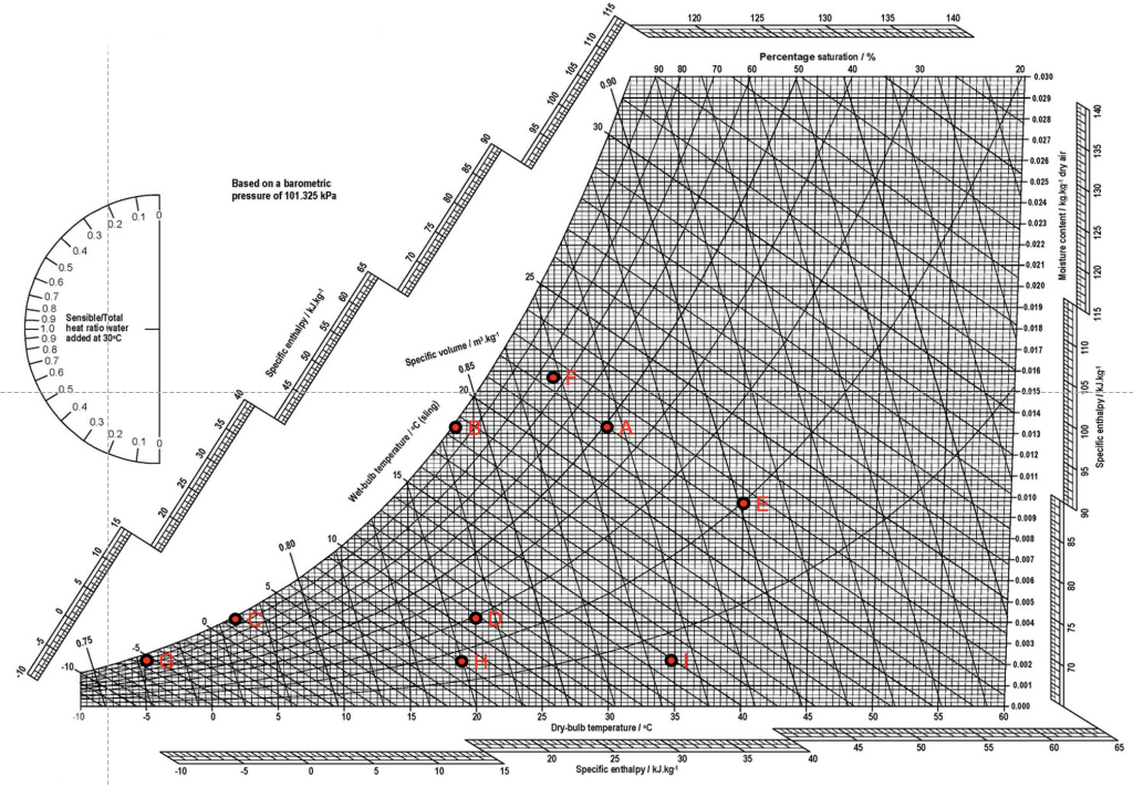
Figure 6: CIBSE chart illustrating some basic psychrometric processes

Consider now an alternative wintertime scenario, in which we have outside air at a state of around -5^oC and 85% relative humidity (point G) and a specific enthalpy of just 1 kJ/kg. We wish to transform the state of this air by raising its temperature and moisture content, again to point D. We must first heat this air to point H (at around 26 kJ/kg), requiring 1.5kW of work to be effected. Next, we add some additional heat in the form of steam to humidify the air, changing its state from H to D, our target supply state, requiring an additional 0.36kW of work so that we effect 1.86kW of work in total. If we consider now a rather unlikely scenario of cooling and humidifying hot dry air at a state (I) of around 35oC and 5% RH and a specific enthalpy of 43 kJ/kg, we would need to perform a total of 1.38kW of work. Finally, let us consider a more plausible scenario of air (say in Arizona) at an initial state E of 40^oC and 20% RH, having a specific enthalpy of 67kJ/kg. We wish to transform the state of this air to 26^oC and 75% RH, state F. We can achieve this by injecting water into the air using a specific nozzle that produces a fine mist of small ( $\sim 30 \mu m$ ) water droplets that quickly achieve full evaporation, thus raising the moisture content of the air. Interestingly, the air at state F has the same specific enthalpy as that at state E – the work that has been done in cooling our air has been achieved by using the latent heat of vapourisation of water. This kind of change of state without a change in enthalpy is referred to as an adiabatic process.

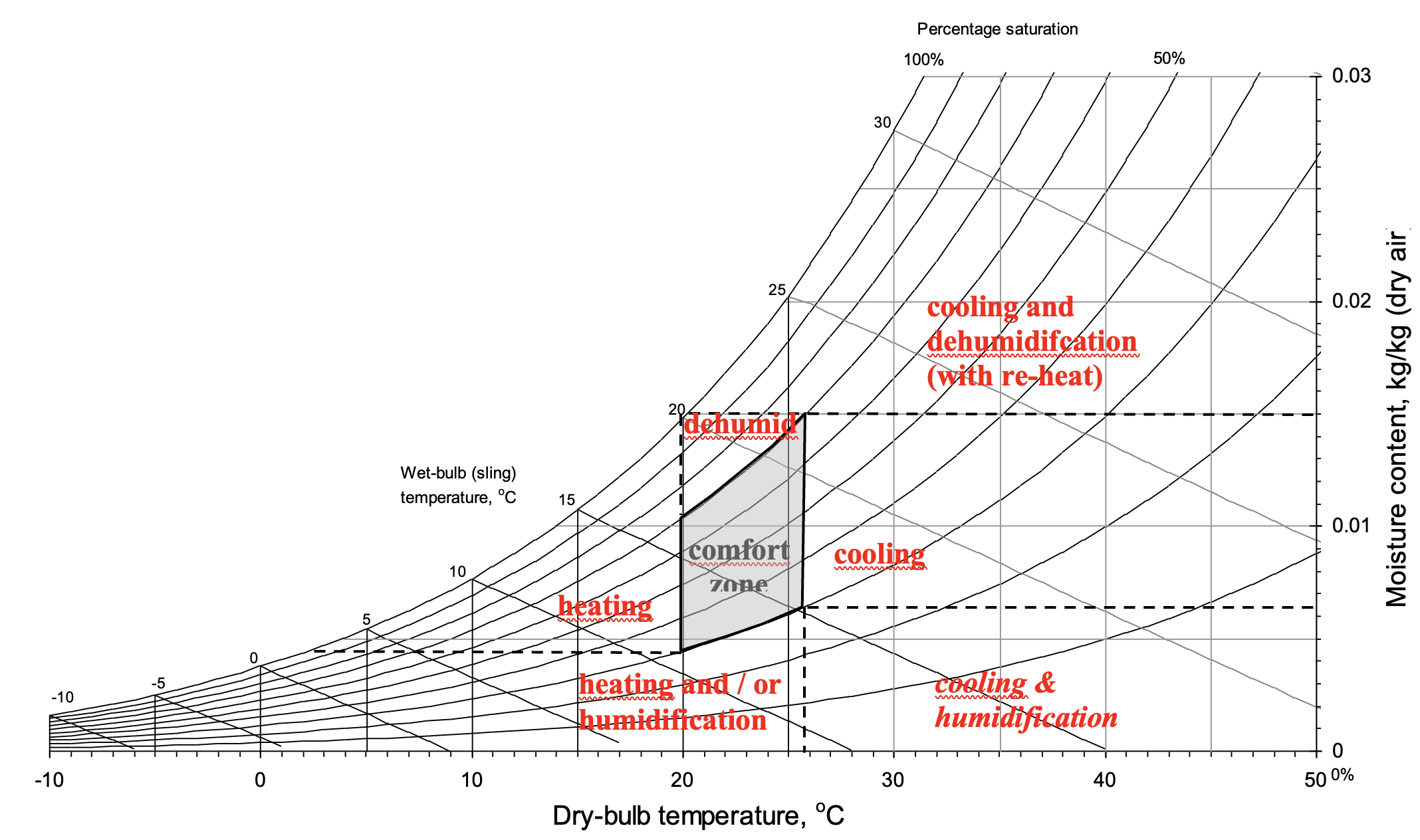
For information, the following simplified psychrometric chart (Figure 7) illustrates a fairly standard comfort zone and regions that correspond to different kinds of air-conditioning process that may be required to condition outdoor air to transform its state to that within the room’s comfort zone.

Figure 7: Psychrometric chart illustrating regions of air-conditioning demand

2.4 Questions and worked examples

This section contains a series of worked examples or problems (P) and their solutions (S), as well as a series of written questions (Q) and their written answers (A).

P1) Shortly after having had a shower, the air in your bathroom has a temperature of 21^oC and a relative humidity of 80%. You look towards a mirror that is fitted onto an external wall and the surface of this mirror has a temperature of 16^oC. Are you likely to be able to see your reflection without wiping the mirror free of condensation?

P2) If the condition of the air in the bathroom in P1 persists for 15 minutes, how much water is likely to condense on our mirror in 15mins, assuming that it is 0.5m wide and 0.6m high?

P3) What if now we are bathing for 30mins in our bathroom, which has an air temperature of 21^oC and a relative humidity of 95%. This bathroom has a 2m wide by 1m high single glazed window with a U-Value of 5.6W/(m²K). It is -2^oC outside, so that the inside surface temperature is 5.2^oC. How much moisture condenses onto this glass surface during this 30min period?

S1) Let’s first of all calculate the saturation vapour pressure for the surface of our mirror. This we do using our expression for $\log_{10}p_s$ . At a temperature of 289.15K the result from our calculation of $\log_{10}p_s$ = 0.259, which converts (since $p_s=10^{log_{10}p_s}$ ) to a value of 1.817 kPa (or 1817 Pa). We can use this same expression to calculate the saturation vapour pressure of our air at 294.15K, which we can then convert to a vapour pressure thus: $p_w = \phi \cdot p_s / 100$ . This gives a water vapour pressure of 1988Pa. Since the water vapour pressure of our air exceeds the saturation vapour pressure of our surface ( $p_w \gg p_s$ ) then our mirror will be covered in a layer of condensation.

S2) Inserting the first the partial pressure of water vapour of air and secondly the saturation vapour pressure when air is cooled to the temperature at the surface of our mirror into the expression for g presented earlier ( $g = \frac{0.62197*p_w}{p_{at}-p_w}$ ) we have moisture contents for the air in our room and air that is saturated at the temperature of our mirror of 0.01245 kg/kg (or 12.45g/kg) and 0.01136 kg/kg (or 11.36g/kg) respectively. Inserting this into a variant of the above equation: $m_w \approx 28.8 (g - g_s) A t$ , where A is the surface area of our mirror (0.24m²) and t is the number of hours of our observation period (0.25h), we find that just 1.85g (or ml) of water has condensed onto our mirror.

S3) Using the same equations as above, we have that P_s = 2486 Pa, P_v = 2361 Pa and the saturation pressure at the temperature of our glass surface is 884 Pa. The air moisture content g is 14.84 g/kg and that of air at the temperature of the glass surface g_s is 5.48 g/kg. Under these circumstances over a quarter of a litre, some 264 g (or ml) of water condenses!

Q1) Which strategies can be employed to reduce the risk of surface condensation?

A1) The first strategy might be to reduce the production ( $\dot g$ ) or retention (through local ventilation near the point of production ( $\dot V$ )) of moisture, beyond that of outside air. An alternative would be to augment the indoor air temperature through heating, which would in turn raise the temperature of the surface(s) on which surface condensation takes place; so increasing $g_s$ . Finally, the thermal performance of the surface could be improved, say by adding insulation in the case of a wall surface, or an additional layer of glass in the case of glazing. This too would increase the surface temperature (and $g_s$ ).

References

Jones, W.P. (1994), A review of CIBSE psychrometry, Building Services Engineering Research and Technology, 15(4), p189-198, 1994.

ISO (2012): ISO 13788:2012: Hygrothermal performance of building components and building elements — Internal surface temperature to avoid critical surface humidity and interstitial condensation — Calculation methods.