
4 Airflow within and around buildings
There are two primary reasons to promote the controlled flow of air within buildings: (i) to meet the fresh air needs of a building’s occupants, and (ii) to regulate indoor air temperature, humidity and pollutant concentrations, to ensure that the indoor environment is thermally comfortable, that the air quality is good and that moisture and temperature (we refer to these as hygrothermal) conditions do not promote condensation as well as fungal or bacterial mould growth.
So, on the one hand, we wish there to be a sufficient flow of air to meet these needs, but not so much as to increase the demand for heating or cooling beyond what is needed. As we know, the vast majority of buildings are assembled from their individual component parts in-situ by a range of craftspeople and their assistants. Some of these component parts contain imperfections, and these imperfections can be introduced during their assembly. This is particularly the case, in the present context, around openings in the envelope, such as around doors and windows; at junctions between wall, floor and roof; and at sites of penetration for ducts, cables and piping. In older properties, there may also be open chimney flues and air-bricks to ensure there is sufficient Oxygen to support combustion in fires. These imperfections lead to the leakage of air through holes, pores, cracks and fissures in the envelope. We refer to this as infiltration. This cannot be dynamically controlled, though efforts can be employed to seal up the sources of air leakage, referred to as draft sealing. Buildings with poorly sealed, leaky envelopes have relatively high infiltration rates and this entails a thermal energy (and potentially a thermal comfort) penalty.
Air infiltration is complemented with air ventilation, whether natural or mechanical. Natural ventilation involves the manual or automated control of ventilation openings in the building envelope, typically windows and doors. Variations in wind pressure around the building envelope in the vicinity of these openings combine with buoyancy pressure differences between indoor and outdoor air (warmer indoor air being more buoyant than cooler outdoor air, or vice versa). These buoyancy and wind pressures drive the flow of air through these openings, which can then be regulated to maintain comfortable indoor conditions.
Alternatively, a building’s ventilation needs can be met by using mechanical ventilation systems, whether or not these are coupled with heating and air-conditioning systems to change the temperature and humidity of the incoming air. In this case, the building is normally ventilated through ducts which connect the intake(s) of a building, through an internal network of ducts, to the outlet(s). Each room within the building similarly has one or more intakes (a supply grill or diffuser) and one or more outlets (return grills or diffusers) which are in turn connected to supply (from intakes) and return (to outlets) ducts. One advantage of mechanical ventilation systems is that they also provide for the possibility of exchanging heat and moisture from the outlet airstream to preheat or (de)humidify the intake air stream, using heat (and moisture) exchangers. These systems are referred to as Mechanical Ventilation with Heat Recovery (MVHR).
Occasionally mechanical ventilation solutions are employed as a backup to natural systems to maintain comfort in more extreme weather conditions. We refer to these buildings as mixed-mode buildings. There are also cases in which heat recovery devices have been incorporated with a building’s natural ventilation pathways, but these are uncommon.
Buildings are of course situated within a rural, semi-urban or urban context. This context, that is the interactions between buildings and other topographical features, including trees and water features, influences the wind microclimate around our buildings. In some circumstances, this can lead to uncomfortably large forces acting on the human body, with adverse consequences for pedestrians’ comfort and even their safety. The wind microclimate also influences the distribution of pressures around openings within the envelope of our buildings, which in turn can influence the naturally induced flows of air through them.
4.1 Introductory fluid mechanics concepts
The airflows that we observe within and around buildings typically travel at low velocities and involve correspondingly low pressures. Under these circumstances, it is safe to assume that the air [1] is what we call incompressible. In other words, the pressure fluctuations are small enough that this alone will not alter the volume that a certain mass of the fluid (air) occupies. For the present, we will also assume that our fluid (again, air) is isothermal. This means that its density does not change and thus also that the volume that is occupied by a given mass of fluid is also unchanged.
Under these circumstances, three forms of energy are present. To explain these, let us first consider a ping-pong ball, which you find sitting immobile on the floor by your feet. If you were to pick up this ball and raise it as you stand up, you would increase its potential energy Epo (strictly speaking, its gravitational potential energy), the product of its mass m, acceleration due to gravity g, and the height that you have raised it, h ( ). This is a little bit like stretching a spring that connects our ball to the floor surfaces. As you raise the ball, you stretch the spring to do so, performing work, as much as you have to perform work to resist the influence of Earth’s gravity by raising it. If you now let go of the ball, our imaginary spring reacts as it attempts to revert to its unstretched state, pulling the ball back to the surface, in much the same way that gravity pulls the ball back to the surface. During its journey in free fall, the kinetic energy Ek of our ball increases as it accelerates towards the floor, the value depending upon its mass m and its velocity v (
 ), where its velocity at the point of impact with the floor would be
  so that the ball’s kinetic energy at this point would be
  : our potential energy has now been fully transformed back into kinetic energy. Our third form of energy is the pressure energy Epr. Let’s assume that when the two halves of our fabricated ball were sealed together, the pressure within the ball at that moment was at equilibrium with the pressure outside of the ball. The pressure exerted on the walls from the inside is equal to that acting on the walls from the outside. However, if we were able to magically remove the air surrounding our ball in an instant, placing it in a vacuum, we would now have more than 100kPa of pressure acting on the inside walls of our ball with no balancing pressure acting on the outside walls, our ball would explode in response to this unbalanced pressure energy (
 )!
)!
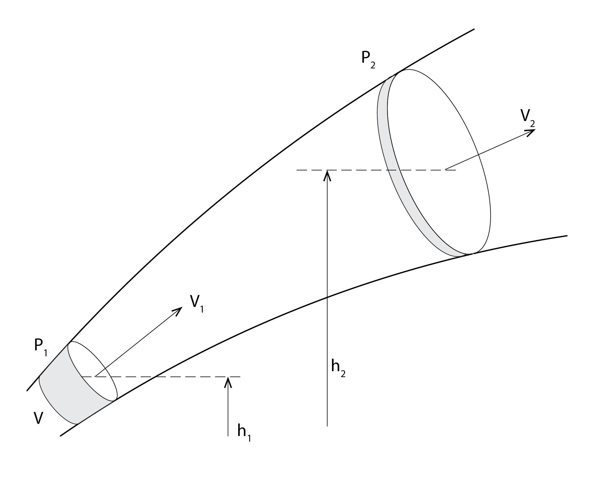
Let us return now to the fluid realm, and the flow of a parcel of fluid of constant mass and volume through a pipe of increasing height and enlarging diameter from position 1 to position 2, as indicated below. Note that the volume V of our parcels at positions 1 and 2 is equal to their average cross-sectional area A and the distance  that the fluid traverses at a velocity v in a time
  , so that
  . So, for our volume to be conserved at points 1 and 2, the increase in area A at 2, must be balanced by a corresponding reduction in the distance our fluid traverses . This derives from what we refer to as the equation of continuity for an incompressible fluid.
With no external influences, the total energy of our fluid is conserved throughout its transport from 1 to 2. As such, we can write the following energy conservation equation:
(1) 
In our case of a constant volume, we can divide these component parts by volume to express our fluid in terms of its density and thus transform energies into pressures (in N/m2 or Pa). This is known as the Bernoulli equation:
(2) 
Now, if our fluid is at rest, so that there is no kinetic energy or pressure, then this simplifies to the Hydrostatic equation:
(3) 
From this, we can also write that:
(4) 
where in our case  , hence the negative sign in (4). This forms the starting point for the stack equation that is used to calculate buoyancy-driven pressures and associated ventilation rates.
4.2 Buoyancy and wind pressures
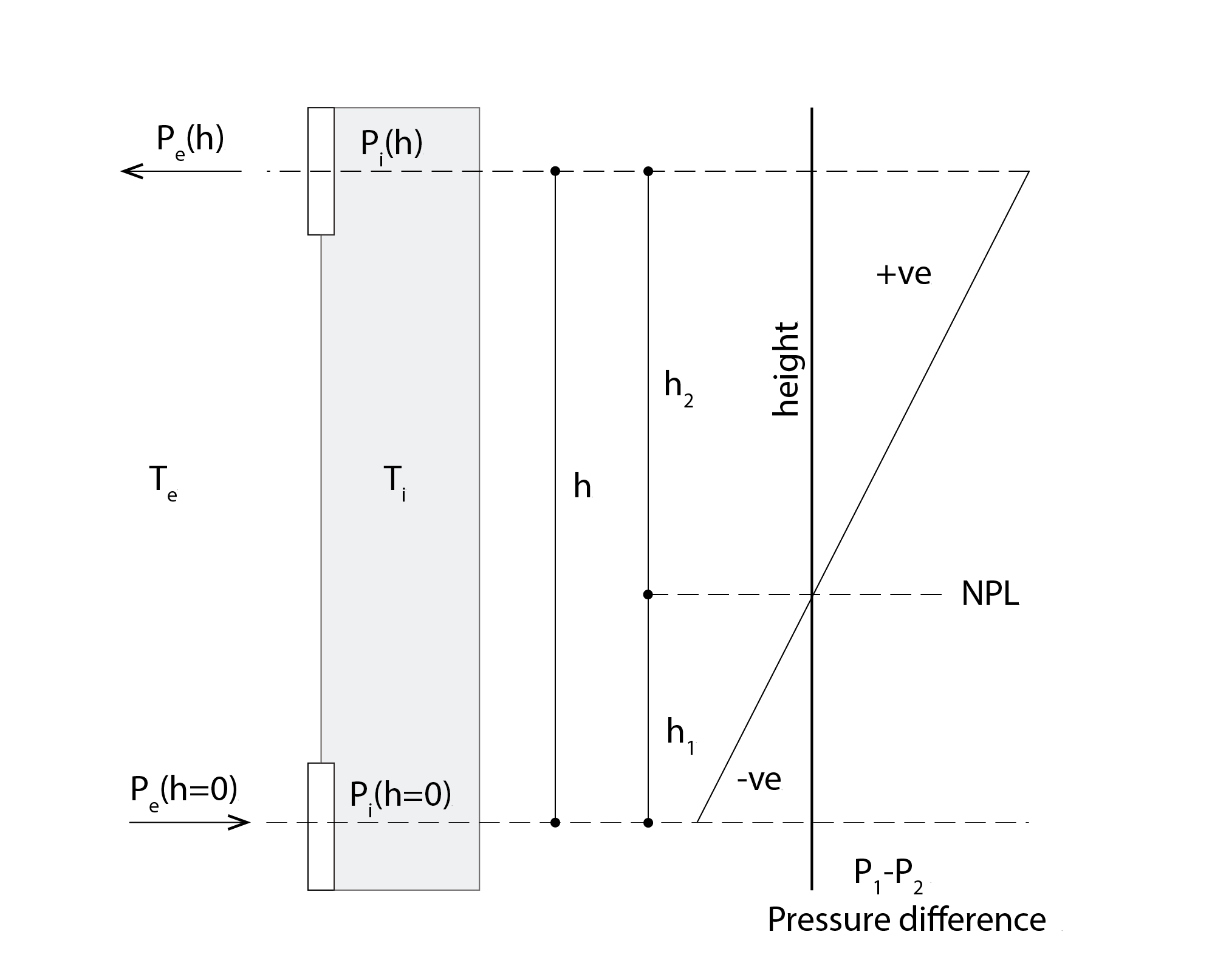
Consider a chimney stack (or say an atrium), with airflow openings at both the base and the top of this stack. There are essentially two columns of air acting on these openings, an external column of air (e) and an indoor column of warmer air (i), so that  and
and  . The density of these two columns is such that we have relatively high-density air flowing into our stack at the base, and relatively low-density buoyant air flowing out at the top (or vice versa, if these temperature differences were reversed).
The graph shown to the right in the image below illustrates pressure differences in the x-axis ( ) and height on the y-axis, extending from the inlet to the outlet. This chart has a positive gradient, passing from a negative region from the inlet, through to a positive region en-route to the outlet, transitioning from negative to positive pressure difference at a location that we call the Neutral Pressure Level (NPL).
Following a similar convention to that established in (4) above, we can write the pressure difference within the stack as  and, equivalently, that outside as
  . The corresponding pressures acting on the two columns i,e at the outlet of the stack are thus:
(5) 
and the corresponding pressure difference (subtracting the pressures from column e from that of column i in 5 above) between the interior and exterior at the outlet is:
(6) 
because  ,
,  are located at the NPL, where
  , simplifying the differences in pressure from equation 5 above. The pressure at the outlet (h) is that at the NPL, LESS the potential energy acting over the head h1, as air is entrained FROM the NPL, driven by the positive
  , so that we do indeed have an outflow at the outlet. In other words, there is a negative pressure acting on the outer plane of the opening into the stack at h.
We can calculate the pressures and pressure differences at the inlet in a similar manner.
(7) 
and thus the pressure difference acting on the inlet is:
(8) 
Now the pressure at the inlet (0) is that at the NPL, PLUS the potential energy acting over the head h1 (hence the positive sign in 7) as air is entrained TOWARDS the NPL, driven by the negative . In other words, there is a positive pressure acting on the outer plane of the opening into the stack at h=0, so that we are subtracting pi(0) from Pe(0) in 8.
The total column of air contained in our stack S is subjected to the sum of the two pressure differences, such that:
(9) 
As noted earlier, this will lead to the standard case of a bottom-up ventilation regime, so long as the temperature within the interior is warmer than that outside, but the inverse will be the case if the inside temperature becomes cooler than that outside, so that we would have a top-down ventilation regime.
Finally, we can slightly reformulate equation (15) to simplify the calculation of our air densities, by making use of a reference air density  , calculated at a corresponding reference temperature
  , so that we have a final form for our total stack pressure difference Δps:
(10) 
where the temperature ratios (e.g.  multiplied by the reference density ) directly determines the density of air at the specified outdoor air temperature (under the assumption of a standard barometric pressure of 101325 Pa).
Now that we know how to calculate buoyancy (or stack) pressures, we can turn our attention to the complementary, and relatively speaking straightforward calculation of wind pressures.
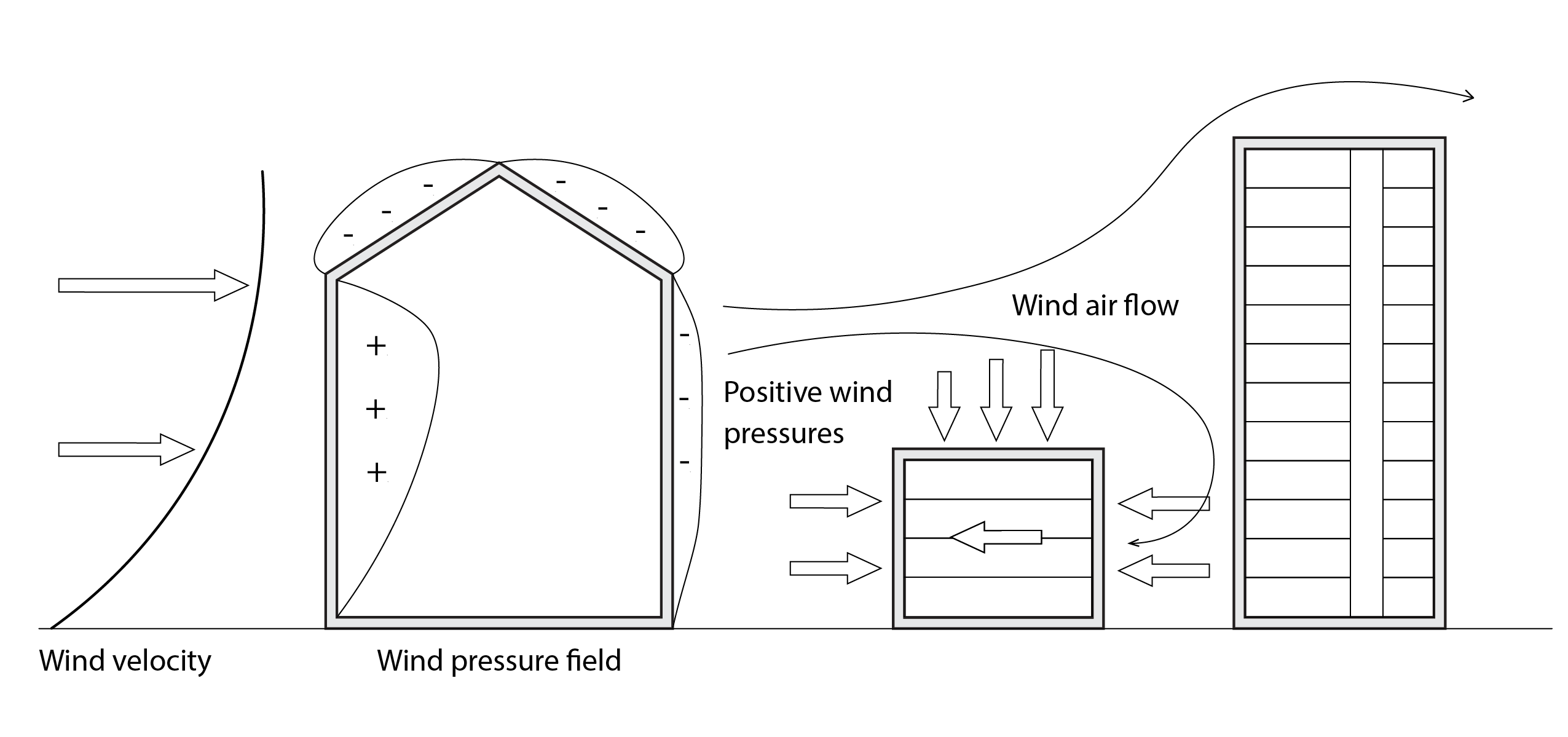
Shown below are two illustrative cases of an isolated building (left) and a relatively small building that is located in front of a taller building (right), with wind approaching the front of our focus buildings in each case. In the isolated case, we see that the wind exerts a positive kinetic pressure on the windward side and a negative kinetic pressure on the leeward side. In the case of relatively shallow-pitched roofs, rather like that shown below, the detachment of air from the windward facade also creates a region of negative pressure around the roof. The positive pressure on the windward facade is complemented by the negative pressure on the leeward facade, acting as a driving force for the flow of air through openings between these facades and thus through the building. In the second case, the down pressure from the tall building creates a back-flow that leads to a positive pressure on the leeward side. This acts to counteract the positive pressure (a little like complementary magnetic poles that repel one another) on the windward side, reducing the driving force for wind-driven airflow through the building. These effects can be accounted for using non-dimensional wind pressure coefficients Cp, normally based on measurements around reduced scale physical models placed in wind tunnels, of which more later.
Using a wind pressure coefficient, the wind pressure acting on an opening can be calculated by multiplying this coefficient by the wind kinetic pressure (the third terms in 2), so that:
(11) 
By re-arranging equation (11), we can also isolate this wind pressure coefficient:
(12) 
This equation is used by technicians operating wind tunnels to calculate average wind pressure coefficients across the facades of scale models of buildings of different size, as noted earlier. They do this by measuring the pressures around the surfaces of the scale model using pressure taps, for different approaching wind directions, at a standard wind speed and temperature, to determine the air density. Similar procedures have been carried out to calculate pressure coefficients of buildings of different proportion that are surrounded by different configurations of neighbouring buildings, which follow structured repeated geometries. Most energy simulation programs contain databases and/or statistical models that have been estimated from wind tunnel measurements, so that these pressure coefficients can be straightforwardly allocated to each relevant window opening. In some cases, particularly where a building geometry is complex, or its adjacent rural/urban topography is complex, it may be necessary to commission the preparation and testing of a reduced scale physical model in a wind tunnel to measure case-specific pressure coefficients (amongst other quantities, for example, related to pedestrian wind comfort).
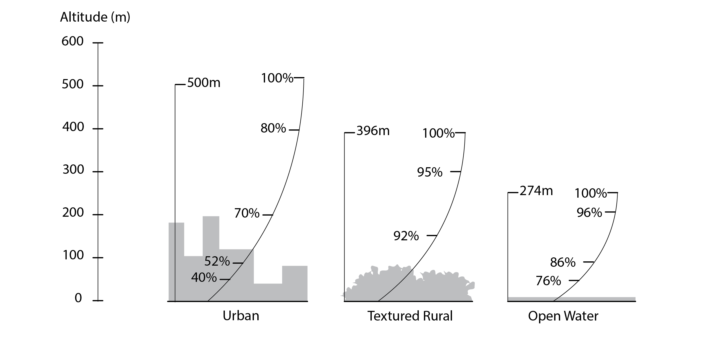
The wind speed that is used in 11 is normally an average wind speed if used as part of a manual calculation or an hourly wind speed if this is calculated on an hourly (or less) basis by a dynamic energy simulation program. In either case, it is often necessary to adjust a wind speed that is measured at a weather station to assemble climate data, these stations often being cited in rural settings (and are typically measured at a reference height of 10m above the ground), to accurately represent the actual site of interest. This is because the surface terrain can have a significant influence on wind speed, hence the need for adjustment. By way of illustration, shown below are three graphs that indicate wind speed relative to the maximum (free stream) speed on x and how this varies with altitude on y. In the open water case, the wind speed reaches its maximum value at 274m above the surface, whereas this increases to some 518m (almost double) in the urban case.
To adjust the reference wind speed ( ), the Charted Institution of Building Services Engineers (CIBSE, 2006) recommend the use of the following equation:
(13) 
where K and a are constants that depend upon the terrain category (presented in the table below) and z is the height at which the reference wind speed is transformed to.
| Terrain category | K | a |
| Open, flat country | 0.68 | 0.17 |
| Country with scattered windbreaks | 0.52 | 0.20 |
| Urban | 0.35 | 0.25 |
| City | 0.21 | 0.33 |
Knowing the wind pressure coefficients on both the windward ( ) and the leeward (
 ) sides of a building, the wind velocity adjusted for height and terrain and the air density, we can now calculate our wind pressure difference Δpw:
(14) 
where  .
.
4.3 Total pressure and ventilation rate
Given our total stack and wind pressure differences, we can now calculate our combined total pressure differences between the inside of our building and its bounding outdoor environment, ΔpT:
(15) 
In practice however, when conducting manual calculations to support initial ventilation design, it is not uncommon to ignore the contribution from wind pressures (our  term), because wind speeds are highly variable and because it is prudent to ensure that the ventilation design will function effectively during calm or still wind conditions.
From either our total (stack + wind) or just the stack pressure difference we can now calculate the velocity of air that would be entrained through our window openings[2] (m/s), as follows:
(16) 
With this we can then straightforwardly calculate the corresponding volume flow rate Q (m3/s):
(17) 
in which A is the area of the ventilation openings (m2) and Cd is a non-dimensional coefficient which effectively represents the efficiency with which the openings support the flow of air through them. The standard value for such an orifice (or opening) is 0.63.
Combining the two, we have the standard form of what is referred to as the standard orifice flow rate equation:
(18) 
where, according to Hunt and Linden (1999) the density  is that of the external air column that is acting on the inlet.
The CIBSE Guide (Volume A) presents a series of equations for calculating airflow rates through different relatively simple building configurations, including multi-floor crossflow ventilation and single-sided ventilation.
4.4 Ventilation design and control
The text in the prior sections of this chapter all leads up to the final presentation of equation 18, with which we can calculate the volume flow rate through a single room, a combination of rooms, an atrium or an entire building, so long as the interior layout is permeable (not blocked off by walls and doors). But there remain some important questions to ask, including how do we determine:
- The volume flow rate that is needed?
- Whether the opening or the ventilation pathway can meet the required effective opening area?
- That the required flow rate is equally delivered throughout the building?
- That this is suitably controlled to deliver the needs for ventilating and cooling?
The remainder of this section is dedicated to answering these questions.
Volume flow rates
As mentioned in the introduction to this chapter, the primary reasons for ventilating a building are to satisfy occupants’ fresh air requirements and to regulate the building’s indoor climate, primarily from a thermal point of view, to ensure that the temperature is not too hot during the daytime in summer and that heat that has accumulated within the structure of the building during the daytime can be effectively discharged at night through night-time ventilation; thereby cooling the fabric by convection.
The CIBSE Guide Volume A recommends fresh air requirements, call these  for what are termed low, moderate, medium and high standards of air quality, corresponding to 5, 8, 12.5 and 20 l/s/person respectively. Given a target number of occupants n for a given space then the corresponding volume flow rate of fresh air that is required to be delivered Q (m3/s) is simply:
  , given that there are one thousand litres per m3.
Concerning the second requirement, experience (of the author) suggests that an air change rate (ACR) of around 5/h [3] is adequate for daytime ventilation purposes, but that this could increase (particularly given the typically larger driving temperature differences) to as much as 10/h for night time ventilation-cooling purposes. This latter figure is higher to promote sufficient discharge of heat and is made possible because occupants are not present (though if they are, the lower daytime maximum would probably be prudent). This can similarly be converted into a volume flow rate as follows:  , where nv is the number of air changes per hour, V is the volume and there are 3,600 seconds per hour.
We thus have an approximate basis for determining our required volume flow rates (both minimum and maximum) with which to evaluate whether our natural ventilation strategy meets these requirements, or alternatively to develop our natural ventilation design concept given these requirements.
Effective opening areas
The standard orifice flow rate equation presented in the previous section, equation (18), includes two related terms, the opening area A and the discharge coefficient Cd. These are often combined, in which case their product is referred to as the effective opening area  . We will come back to this later, but first, let’s examine the discharge coefficient in more detail.
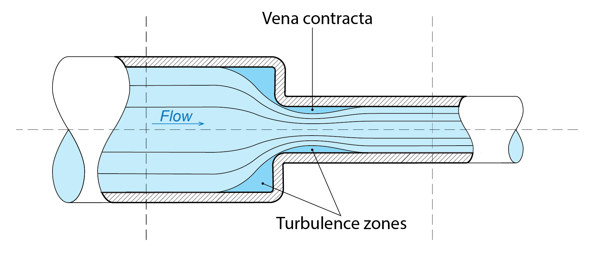
Shown below is an image of a pipe that has an abrupt reduction in its diameter. This constriction behaves in much the same way as the plane of an unobstructed window opening (i.e. the window is fully open) on a building facade. As the diagram illustrates, two symmetric turbulent regions are created by the constriction. One on the left side above and below the entry to the constriction and a further on the right side, within the throat, just after the entry. Now, on the left side, we observe a series of parallel streamlines, indicating a smooth laminar flow. The constriction causes a change of direction of these streamlines, generating eddies that lead to the development of the two turbulent regions. Within the throat, the diameter that corresponds to relatively smooth flow is smaller than the pipe diameter, due to the developed turbulent regions. We call this the vena contracta. The diameter is essentially contracted, reducing the effective opening area of the plane of the opening into the narrower pipe (analogously, reducing the plane of the window opening).
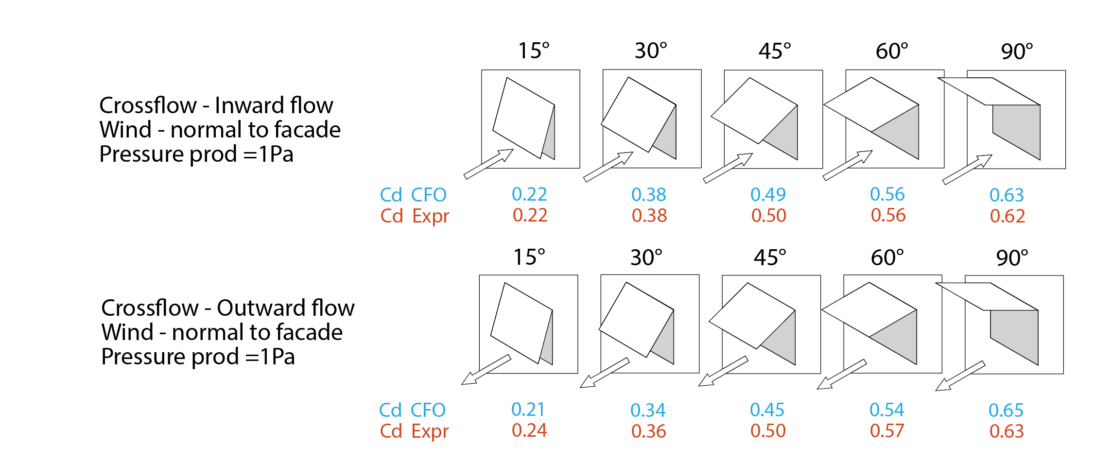
The image below depicts experimentally and numerically derived values for the discharge coefficient for different combinations of window opening proportion (or aspect ratio) and for different angles of opening of the top-hung window. The numerical and experimental results coincide very well (giving confidence in the former). More important in the current context, however, is the observation that the discharge coefficient is only moderately affected at an opening angle of 45o and above, but drops off rather rapidly below this value, as the window impedes the path to the plane of the facade opening.
In buildings that are likely to be ventilated predominantly by wind pressure, particularly buildings that are subjected to cross ventilation, in which one facade is connected to another, potentially through intervening openings such as doorways, the effective opening area may need to be calculated for the combination of these windows. This can be performed using the following equation, for each j of a set of n openings:
(19) 
Occasionally, natural ventilation designs in buildings are not as simple as a plane window opening. Sometimes they involve a flowpath with a combination of elements, each of which causes a drop in pressure. For example, an inlet opening may contain controllable dampers, supplying air to ducts, potentially then supplying air to an array of parallel ducts created by acoustic absorbers before then supplying air to a room via a supply grill. This then has parallels with standardised mechanical ventilation systems. Fortunately, there are standard coefficients that have been experimentally determined for a vast range of these kinds of ventilation system components and we can call upon these to calculate an effective opening area. These are published by the CIBSE, in Volume C of The CIBSE Guide.
These velocity pressure loss coefficients  are calculated by experimentally measuring the pressure (p) drop across the component, the velocity (v) of the airflow upstream of the component and the air density (). The coefficient can then be calculated as follows:
(20) 
The velocity pressure loss coefficient and the discharge coefficient  are related to one another. Firstly, we know that
  (m/s). It follows then that
  and that by re-arranging equation (20),
  . Therefore, it follows that:
(21) 
So, if we can calculate a combined value of for each of a set of components along a complex flowpath, then we can also calculate its equivalent discharge coefficient and thus its effective ventilation opening area. Fortunately, doing so is relatively straightforward[4]. This simply involves the following steps:
- Choose a reference volume flow rate of air, say 5m3/s.
- For each component, calculate a local entry velocity v, simply the volume flow rate Q over the total entry face area A.
- Using published values for calculate the local pressure drop or loss:

- Now calculate the total system velocity pressure loss coefficient for each of the j components:
 , where v is now the supply velocity, calculated as in 2 above.
 - Now calculate the effective discharge coefficient:
 .
.
The total effective ventilation area is then simply:  . This may seem a little cumbersome, but it is a really convenient way of being able to manually calculate complex natural ventilation problems. In cases where published values of are not available, it is possible to employ Computational Fluid Dynamics (CFD) software – of which more in section 4.6 – to calculate them.
Balancing of ventilation provision
An important feature of the stack model presented in section 4.2 is that the position of the NPL does not affect the magnitude of airflow through the stack, but it does affect whether we have either an inflow or an outflow at a particular position within the stack, which of course may span multiple floors in real buildings. It is important then, to design our airflow openings in such a way as to ensure that the NPL is located high enough within the stack so that there is only an outflow where this is intended, that is, above the uppermost occupied floor. This can be achieved by ensuring that the total outlet opening area is at least equal to the sum of the inlet effective opening areas, and also that the outlet is located sufficiently high above the uppermost occupied floor, preferably one storey height above.
Now, if we inspect equations (10, 15 and 17), we can write that:
(22) 
It should be apparent then, that if we express the incoming velocities through two different floors (1 and 2) feeding a stack in a building, expressing these as a ratio, that:  and that
  . In other words, we can balance our volume flow rates simply using the square root of stack heights relative to a reference height, say the stack height to the lowest floor that feeds the stack.
Despite the fact that wind speed increases with height, wind-driven pressures tend to drive lateral rather than vertical flows. In other words from one side of a building to another rather than up through the building. As such, we don’t tend to concern ourselves with wind pressures when vertically balancing window openings.
Ventilation control
In the case of residential buildings in particular, but also in the case of smaller relatively straightforward non-residential buildings, ventilation openings tend to be manually controlled. Even under this scenario, it is all too often the case that window openings are specified that do not offer sufficient control over the elements (e.g. rain or gusts of wind) and/or that do not offer sufficient control of opening angles. Sometimes windows that tilt inwards take up too much internal space to provide sufficient opening angles and some windows simply offer too much mechanical resistance to open – sliding windows are often a case in point. It is important then that windows that are manually opened are designed in such a way that the mechanism is obvious to the user and that the required degree of open-ability is easily offered and in a way that protects adequately from the elements.
One reason that manually controlled window openings are particularly well suited to residences, is that households feel uninhibited in using them for their purposes. Some negotiation with other household members may be needed but this tends to be more straightforward than with other colleagues, particularly where power structures are at play. Another is that household members often develop window opening (and other forms of adaptive control) strategies that are very sophisticated and very well suited to their needs, albeit through trial and error.
In non-residential buildings, particularly those that accommodate staff in open-plan layouts, where high solar and internal casual heat gains may be involved and where internal pollutants may also be present, some level of automation of ventilation opening control is desirable.
The fresh air requirements presented in the Volume Flow Rate section above relate to the achievement of acceptable levels of Carbon Dioxide concentration in the workplace. The same categories of Low, Moderate, Medium and High standards of air quality relate in this case to maximum acceptable concentrations of 1600, 1200, 900 and 750 parts per million (PPM). CO2 sensors can be installed and linked to Building Management Systems (BMSs) which are linked in turn to mechanical or electrical actuators fitted to window (or the ventilation) openings, usually ramping from some lower concentration up to this maximum concentration, to ensure that the interior is sufficiently flushed of indoor pollutant. Classrooms are interesting cases where during a lecture there may be high occupancy levels, each occupant respiring CO2, so that concentrations may exceed the above limits. In this case, it is common to flush the room either by opening windows to a large or to their maximum extent or by running mechanical fans in a boost mode.
Of course, CO2 isn’t harmful to humans in itself, but it can be a good proxy indicator of inadequate levels of Oxygenation as well as of the presence of other forms of pollutants. One issue with CO2 sensors is that they are expensive, as they use relatively sophisticated technology to measure the absorption of infrared radiation (band absorption) – the extent of absorption being proportional to CO2 concentration. In some cases, they can also be prone to calibration drift, meaning that their accuracy can deteriorate over time.
Increasingly, packaged sensors that measure a range of pollutants are available and can also be connected to Building Management Systems. Examples of parameters measured by these sensors include Particulate Matter (PM) in different sizes, typically 2.5  in diameter and 10 , measured in
  , volatile organic compounds (VOCs) measured in or PPB, Ozone (O3) and Nitrogen Dioxide (NO2), both measured in PPM and PPB. At high concentrations, these pollutants PM, O3 and NO2 can cause respiratory disease, while high concentrations of VOC can be an allergen, increasing the risks of occupants developing asthma symptoms. Causes of VOCs include paints, aerosol sprays and wood preservatives; NO2 is mainly a by-product of combustion from equipment that is inadequately ventilated; O3 tends to be produced by electrical equipment such as photocopiers and laser printers; Particulate Matter can be generated as a combustion by-product and also as a result of smoking, though the main source is from outdoor air that contains particulate matter produced by the erosion of tyres and the exhausts of internal combustion engines, diesel especially. Finally, ventilation is also required to expel excess levels of moisture from the air, particularly in close proximity to sources of moisture production, such as kitchens and bathrooms. It is commonplace now to install extractor hoods above cookers to remove excess moisture and cooking-related smells. It is also common, and indeed a Building Regulations requirement, to install extract fans in toilets and bathrooms, to expel excess moisture and smells; the former, being particularly effective in reducing the risks of surface and interstitial condensation.
A useful article discussing the accuracy and long-term reliability of air quality sensors is available here.
As hinted at above and explicitly mentioned in the introduction, the other main reason to ventilate buildings is to reduce excess heat build-up during warm daytime periods and to discharge at night excess heat that has been stored within the building fabric during the daytime. The former is relatively straightforward, with the opening proportion being some function of a maximum (Tmax), minimum (Tmin) and current (T(t)) air temperature, such as:  , while
  .
.
Night-time cooling is more complex, as this ideally requires some mapping between the state of the air (Ta) and the state of the fabric or structure (Ts). One approach is to embed a temperature sensor directly within an element of the building fabric, for example within a concrete floor, either by placing and sealing the sensor within a drilled hole in the case of pre-cast concrete, or by carefully placing a sensor within formwork, to be encased in concrete when it is poured in-situ. Some overheating setpoint air temperature (T’a) can then be mapped onto a coincident structure temperature (Ts‘), with night cooling being activated whilst  , and continuing until
  , potentially using some adjustment f to this mapping, perhaps using a self-learning algorithm.
4.5 External airflow and comfort
The 1960s and 1970s bore witness to a vast international programme of developing high-rise housing solutions as well as office blocks and multi-use buildings within urban centres and peripheries, with relatively little understanding of the social and physical impacts that these developments would have. Amongst these impacts was a wave of incidents involving wind-blown debris falling from these towers and hitting objects and people at ground level, as well as pedestrians being literally blown off their feet. Less extreme, but still considered unacceptable, was a feeling of (sometimes profound) discomfort arising from gusts that were created from the injudicious proportions and placements of these towers. This promoted a plethora of studies into the mechanical wind comfort of pedestrians and a corresponding suite of criteria against which to judge (dis)comfort. These are summarised in the diagram below (after Robinson, 2011).
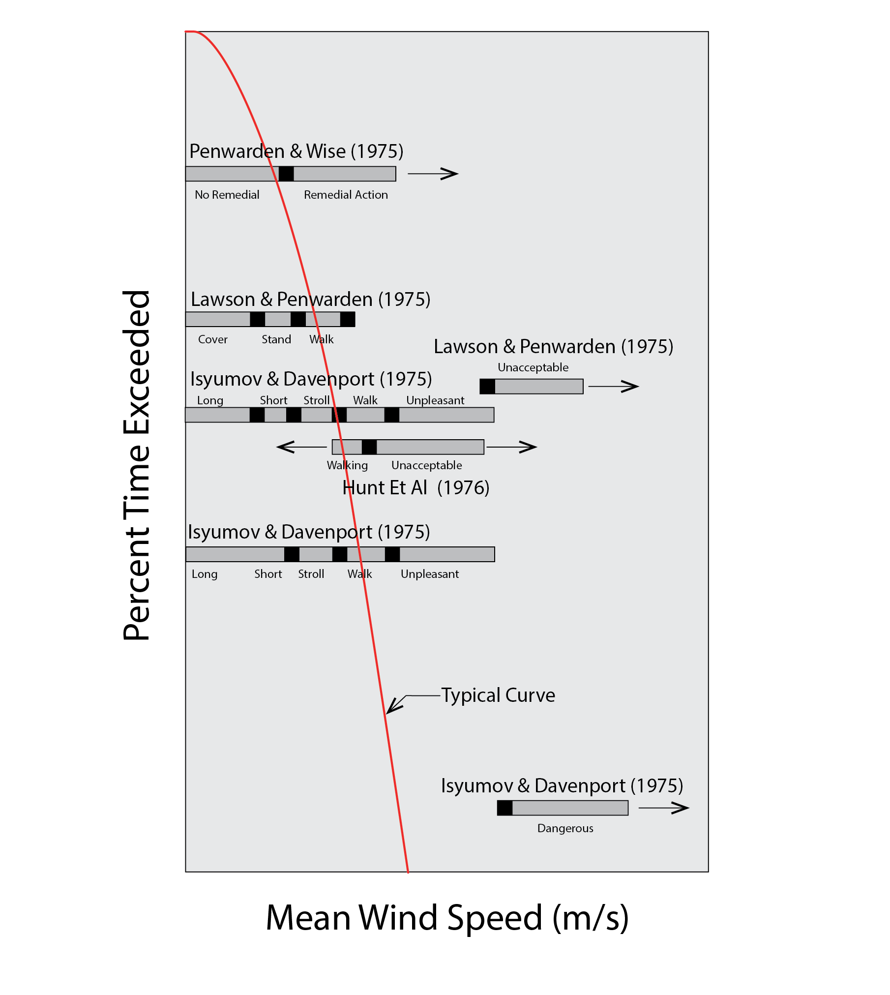
Of these, the criteria of Lawson and Penwarden have found widespread use in practice. These are expressed in the following table with respect to unacceptable and tolerable thresholds of exceedence of wind speed expressed on the Beaufort scale. Wind tunnel modelling (see section 6 below) is normally employed to evaluate whether the criteria mentioned below are met or not for a given type of activity.
Lawson’s pedestrian wind discomfort criteria
Description
Letter
Threshold of exceedence considered unacceptable
Threshold of exceedence considered tolerable
Roads and car parks
A
6% > B5
2% > B5
Business walking
B
2% > B5
2% > B4
Pedestrian walkthrough
C
4% > B4
6% > B3
Pedestrian standing
D
6% > B3
6% > B2
Entrance doors
E
6% > B3
4% > B2
Sitting
F
1% > B3
4% > B2
The Beaufort scale was introduced in 1806 by Admiral Sir Francis Beaufort in an attempt to standardise the perceived effects of wind in relation to different levels of magnitude, from 1 to 9. These are expressed in the table below.
The Beaufort wind scale and its qualitative effects
Beaufort Number
Description of wind character
Mean wind speed, m/s
Qualitative effect
0
Calm
0 – 0.24
Calm (smoke rises vertically)
1
Light air
0.25 – 1.54
No noticeable wind (smoke drift indicates wind direction)
2
Light breeze
1.55 – 3.34
Wind felt on face (leaves rustle)
3
Gentle breeze
3.35 – 5.44
Hair disturbed, clothing flaps and newspapers difficult to read
4
Moderate breeze
5.45 – 7.94
Hair disarranged (raises dust and loose paper)
5
Fresh breeze
7.95 – 10.74
Force of wind felt on body (small trees in leaf begin to sway)
6
Strong breeze
10.75 – 13.84
Inconvenience when walking (larger tree branches moving, whistling in wires)
7
Near gale
13.85 – 17.14
Resistance felt walking against the wind (whole trees in motion)
8
Gale
17.15 – 20.74
Difficulty in balancing (slight structural damage may occur)
9
Strong gale
20.75 – 24.45
People blown over (structural damage)
4.6 Modelling techniques
A range of modelling techniques have been developed to support the analysis of building ventilation strategies and the evaluation of their effectiveness. These can be broadly categorised into physical and computer models. Physical modelling techniques have been developed to separately support analysis of buoyancy- and wind-driven airflows; the former using salt bath modelling (though this has also been adapted to model wind-driven flows) and the latter using wind tunnel modelling. Computer modelling techniques can model either type of flow problem. These can be categorised as either bulk airflow models (usually co-simulated with dynamic thermal models) or by computational fluid dynamics, which support spatially very detailed analyses and associated visualisations of flow. These are described in brief below.
Salt bath modelling
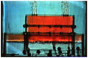
Salt Bath Modelling involves the use of a reduced scale model of an enclosure, usually constructed in perspex, which is immersed upside down in a water bath. A dyed saline solution is injected at the location of internal heat sources, typically due to occupants. The concentration of salt in the saline is adjusted to represent the magnitude of the heat flux. When injected this denser saline solution descends through the model and flows out at the location of ventilation outlets, with clear distilled water flowing into the model at the location of inlets. This incoming clear water is entrained into the plumes that are generated above the point sources of heat at the locations where the dyed saline is introduced (typically at floor level). Steady-state solutions are reached when a clearly demarcated interface develops between the clear and dyed water solutions, representing the neutral pressure level (NPL). The location of this NPL can be adjusted by manipulating the sizes of the ventilation openings. Examples of experimental results compared with theoretical predictions are presented in the ground-breaking paper by Linden et al (1990), from which the following image of the flow through a modelled courtroom is derived.
This is a powerful technique, but it does rely on specialist equipment and the relatively time-consuming construction (and subsequent manipulation) of physical models, so computerised techniques tend to be favoured in practice. It also suffers from the drawback that indoor air and surface temperatures are assumed to be identical, so that the corresponding transfers of heat (which in practice can be considerable) are not accounted for. Nevertheless, this technique has been used extensively in research applications.
Wind tunnel modelling
Wind tunnels employ large fans to circulate air within a kind of corridor in which a reduced-scale physical model is situated. These models are normally placed on a circular rotating platform which is equipped with sensors that are capable of measuring forces to facilitate the calculation of drag and lift coefficients (the extent to which a model resists the flow of air, or causes an uplift (or down-lift)). These wind tunnels employ either open or closed designs. In either case, internal or external air is entrained by a fan into louvres, after which it passes over baffles to ‘straighten’ the incoming air, before entering the corridor. The floor of the approach to the domain containing the physical model is usually covered with blocks that mimic the roughness of the terrain that is upwind of the modelled building for each given wind direction. The model itself normally contains pressure taps to measure the pressure (linking the inlet of a thin tube to a pressure transducer) and hot wire anemometers to measure the air speed. At each location a velocity ratio can be calculated: the ratio of the local velocity to that which enters the modelling domain. This process is typically repeated for each of 16 (22.5o increments) wind directions.
In the case of closed wind tunnels, a recirculating loop is employed, normally involving a corridor above that which supplies the modelled domain, to return air to the ‘entry’ louvres. In the open case, there is no such recirculation.
In addition to physical measurements, flow can be visualised using smoke, sometimes using a laser sheet that is formed by manipulating a laser beam using a combination of convex and concave lenses. A technique called particle image velocimetry is also sometimes used. This involves the use of tracer particles of small diameter (10-100 )) that have a similar density but a different refractive index to air, so that they can be visualised in a very high speed video of the experiment. Image processing techniques can then be employed to calculate, based on the position of the same particles in adjacent video frames, the velocity of these particles, providing rich quantitative information describing the characteristics of the flow field.
Bulk airflow modelling
As noted in Chapter 1 on “Heat, Temperature and Thermal Energy”, a bulk airflow network can be created in which internal air nodes correspond with the nodes of zones in a thermal model. The thermal model then provides temperature input to the airflow network, as well as the coincident wind speeds at external air nodes. This information can be used to calculate the wind and buoyancy pressures and the corresponding mass flow rates (essentially solving the equations presented earlier in this chapter) at each node in the network, feeding this back to the thermal network for a revised calculation of the internal air temperatures and so on, until the two modelled domains reach a solution that satisfies some convergence criteria.
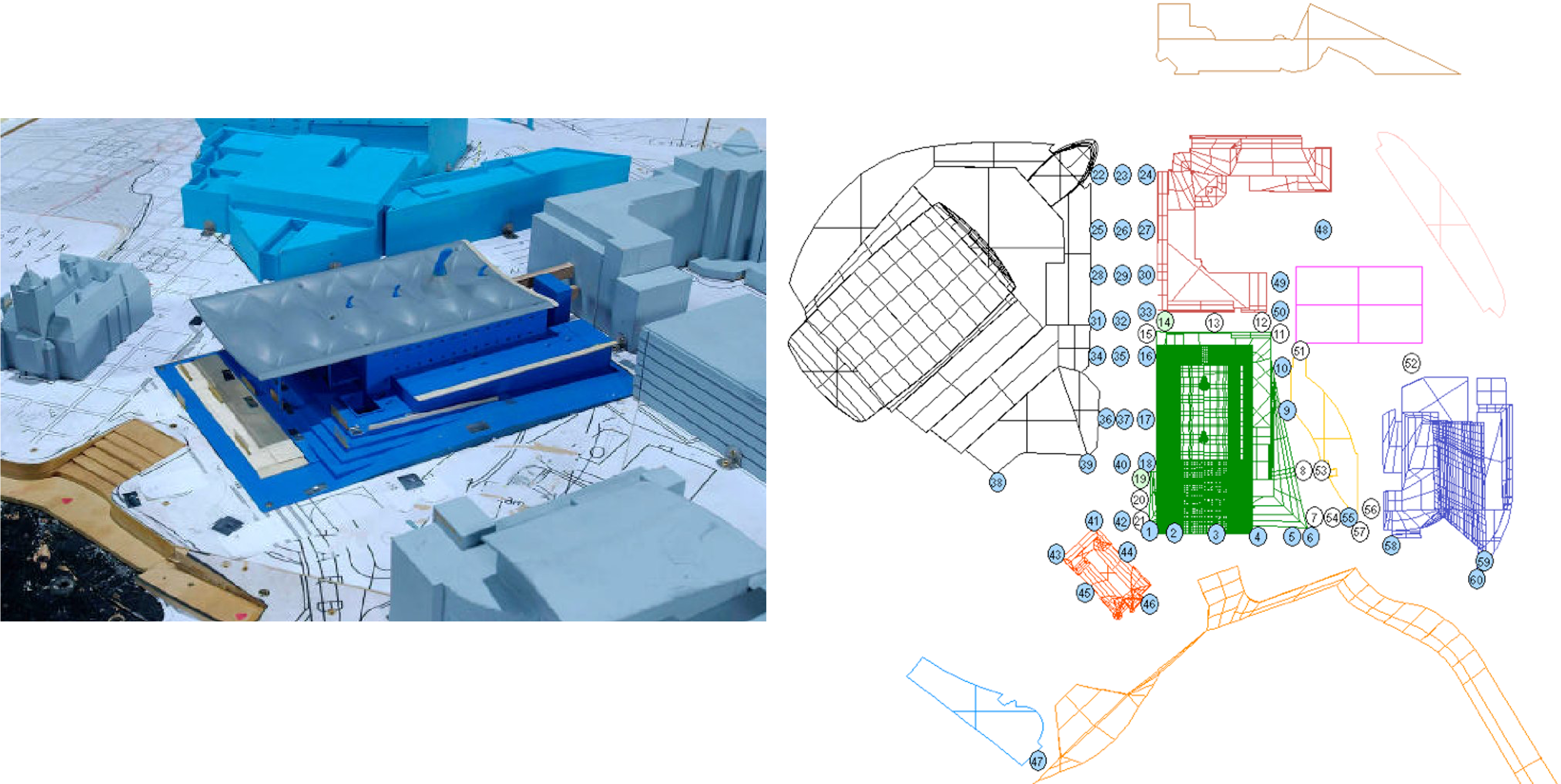
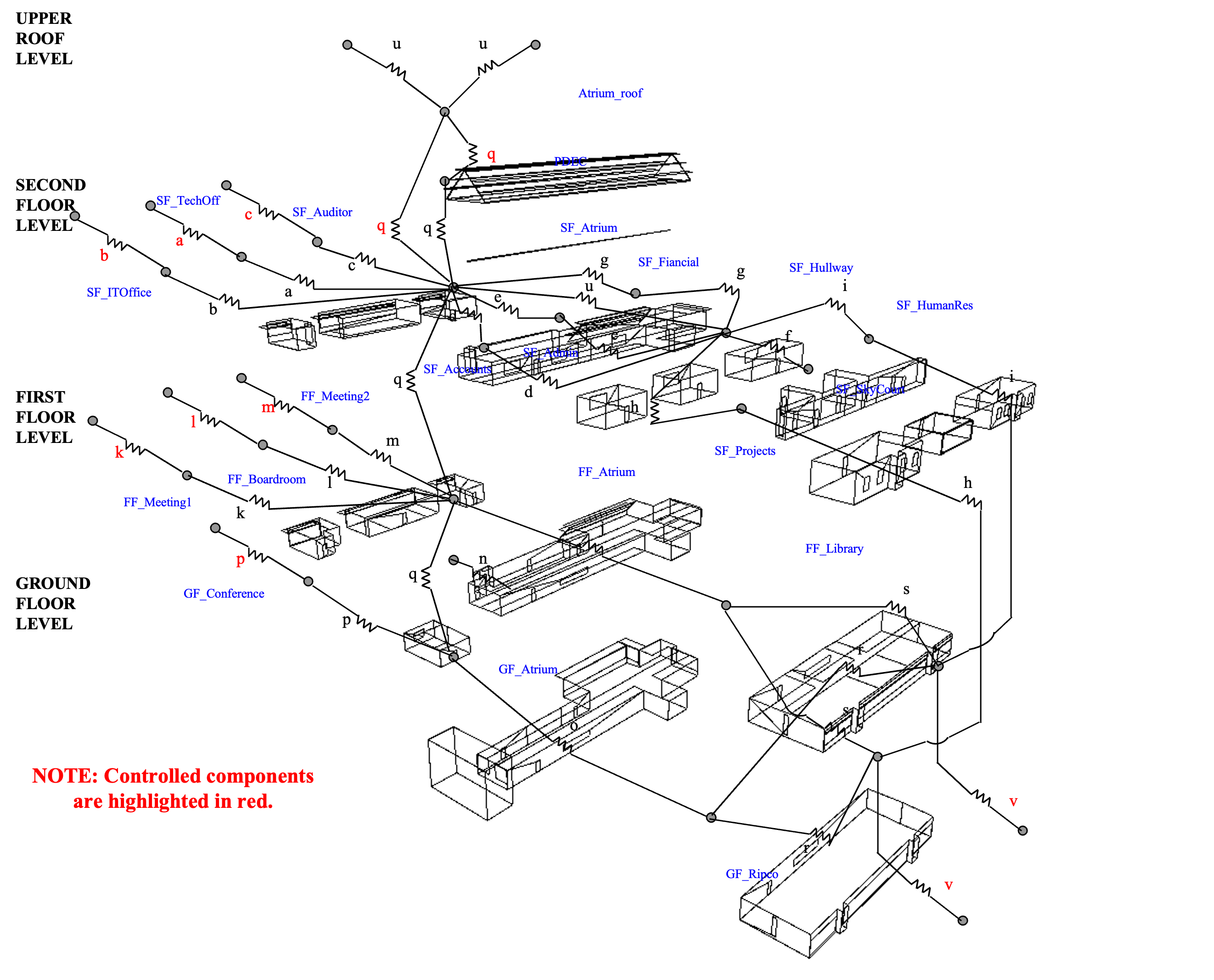
Shown below is an example of a thermal model network (lines describing the edges of the faces of surfaces that bound a 3D volume of each modelled zone), exploded in this case to facilitate visualisation of the model, upon which an airflow network is superimposed. This airflow network is comprised of nodes (shaded circles here), that are connected to one another via flow components (ventilation openings that are indicated by resistors) using simple lines.
Computational fluid dynamics (CFD)
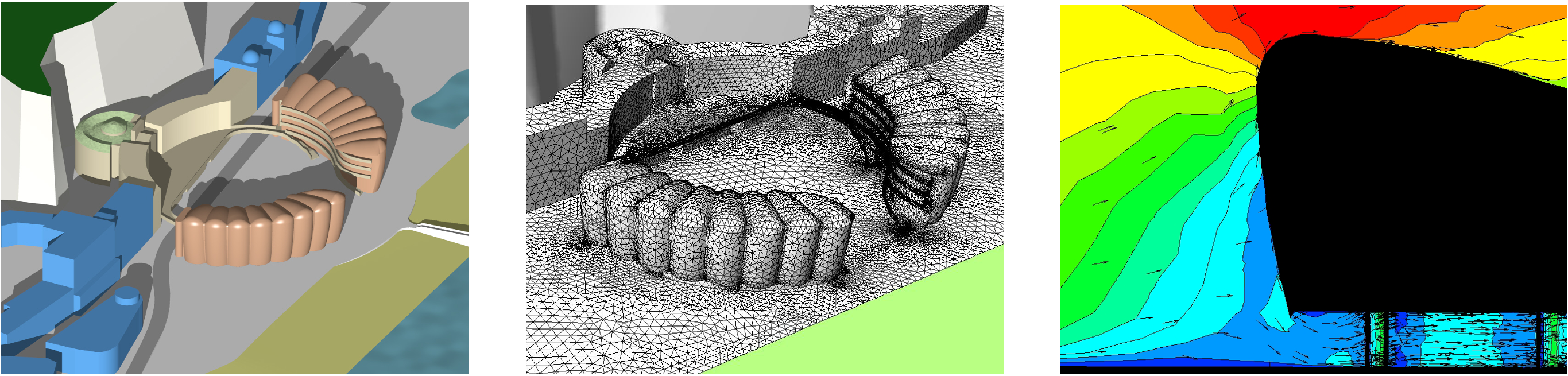
Last but far from least, we have computational fluid dynamics software. With this software, a three-dimensional B-Rep model of a computational domain is first produced. This is normally a large cuboid, where the length, width and height are around five times larger than the corresponding dimensions of the target building(s) to be modelled. The outer geometry of this building (and any other significant local objects) is extruded up from the ground, as shown in the image to the left in the sequence below. A surface mesh is then generated for the ground and the surfaces that are extruded up from it – shown in the centre of the sequence below. This is normally what we call an unstructured triangular mesh, with smaller triangles located in close proximity to surfaces of the building of interest and any points of detail around it. A three-dimensional mesh is then generated from this surface mesh, so that the entire computational domain is associated with one of the resultant three-dimensional cell volumes. The physical surfaces of the modelled target building are then associated with boundary conditions, in particular with a temperature. One or more of the domain walls are then associated with an inflow velocity, which may employ a model of velocity that increases with height from the floor. Similarly, opposing surfaces are also designated as outlets.
Once the model is complete and all the simulation settings have been specified (including parameters that influence the subsequent calculations) the simulation is launched. This involves solving a set of complex three-dimensional conservation equations, called the Navier-Stokes equations for the conservation of energy, mass and momentum (as well as concentration, if pollutant dissipation is also to be simulated). Once a converged solution has been achieved, the results can be visualised. Shown to the right in the sequence below are pressure contours with superimposed velocity vectors. In this case, these are unit vectors, where the tails of the arrows have the same length but their density indicates the speed and their orientation the direction of flow.
CFD modelling is very powerful, but it is also complex and very computationally demanding; though this is becoming less significant owing to the availability of hardware acceleration and cloud computing infrastructure.
4.7 Questions and worked examples
This section contains a series of worked examples or problems (P) and their solutions (S), as well as a series of written questions (Q) and their written answers (A).
P1) A three-storey office building has a floor-to-ceiling height of 3.2m. The mid-point of each inlet is 2m above the floor and the mid-point of the outlet at the top of the central atrium that is served by each occupied floor is located at 2m above the uppermost ceiling. Given that the outdoor air temperature is 15oC and the indoor air temperature is 25oC, calculate the stack pressure for the windows located at Ground Floor level. The reference density and air temperature are 1.1614 kg/m3 and 300K respectively.
P2) A top-hung 2m x 1m window is open at an angle of 60o on the Ground Floor of the building described in 1) above. Calculate the volume flow rate through this opening as well as the mean incoming air velocity.
P3) An office building is ventilated by cross-flow ventilation. The pressure coefficients on the windward and leeward sides are 1.35 and -0.35 respectively. Given that the outdoor air temperature remains at 15oC, calculate the wind-induced pressure difference across the building’s openings for wind speeds of 1.5 and 4.5 m/s respectively.
P4) For the high wind speed case in 3) above, calculate the total pressure difference (that of the wind and the stack from 1) above) as well as the volume flow rate.
P5) A floor of a building is ventilated by cross-flow ventilation. The inlets and outlets are each 2.5m2 in area, and these two are connected by an open door measuring 1.9m high and 1.1m wide. Each opening has a discharge coefficient of 0.63. Calculate the combined effective opening area.
P6) A ventilation component has a measured velocity pressure loss coefficient of 3.25. Calculate the equivalent discharge coefficient.
S1) The total effective stack height between the inlet and outlet is (3.2 x 3 + 2 – 2) 9.6m. Using equation (10) the stack pressure difference is 3.82 Pa.
S2) Based on the experimental results presented in section 4, the discharge coefficient for this opening is 0.56. Using equation (18) the volume flow rate is 2.87m3/s and the incoming air velocity (from equation (16)) is 2.56 m/s.
S3) The wind pressure coefficient difference is 1.7 and the outdoor air density is 1.209 Pa. The corresponding wind pressure differences are 2.31 and 25.69 Pa for the low (1.5 m/s) and high (4.5 m/s) wind speed cases respectively.
S4) The total pressure difference resulting from the combination of wind pressure difference for the high-speed case in 3) and from the buoyancy pressure difference from 1) is 29.5 Pa. The corresponding incoming air velocity is 7.83 m/s.
S5) The total effective area resulting from the combination of the three openings and their respective discharge coefficients is 0.85m2.
S6) Using equation (21), the discharge coefficient for a ventilation component having a value of of 3.25 is 0.555.
References
CIBSE (2006), CIBSE Guide, Volume A.
CIBSE (2007), CIBSE Guide, Volume C.
Hunt, G.R. Linden, P.F. (1999), The fluid mechanics of natural ventilation-displacement ventilation by buoyancy-driven flows assisted by wind, Building and Environment, 34 (1999) p707-720.
Lawson, T. V. and Penwarden, A. D. (1975), The effects of wind on people in the vicinity of buildings, in Proc. 4th Inc. Conf. Wind Effects on Buildings and Structures, Cambridge University Press, Cambridge, pp605–622
Linden PF. Lane-Serff GF, Smeed DA (1990). Emptying filling boxes: the fluid mechanics of natural ventilation. J Fluid Mech 1990;212:300-35.
Robinson, D (2011), Computer modelling for sustainable urban design, Taylor and Francis, 2011.
Further reading
Awbi, H.B. Ventilation in Buildings, Routledge 2003 (2nd Ed).
CIBSE Applications Manual 10 (AM10): Natural ventilation in non-domestic buildings, CIBSE 2005.
Etheridge, D., Sandberg, M., Building ventilation: Theory and measurement, John Wiley and Sons, ISBN 0 471 96087 X, 1996.
Feustel, H.E., Raynor-Hoosen, A., Fundamental of the Multizone Air Flow Model – COMIS, Technical Note AIVC 29, 1990.
- Note that in what follows we treat air as a fluid, much as we would water. Of course, air is a gas not a liquid, but when dealing with its motion these non-solid weakly-coupled (liquid) or un-coupled (gas) collections of molecules behave similarly. ↵
- assuming that this opening is sufficiently small that we can ignore buoyancy-driven pressure variations along its height ↵
- The air change rate (ACR) corresponds to the number of times that the entire internal volume of air has been exchanged with the outdoor environment, during a period of one hour. It is expressed in air changes per hour, sometimes referred to as ACH. ↵
- This methodology was developed to support the ventilation design of the Welsh Assembly building ↵
