Heat, temperature and thermal energy

Darren Robinson

1 Heat, temperature and thermal energy

1.1 Introduction

At its most primitive level, the purpose of a building is to provide shelter, to protect its occupants from climatic extremes and to support them in the attainment of thermal comfort. The envelope of modern buildings is comprised of both opaque and transparent parts. The opaque parts include the floor, walls and roof and this is typically where thermal insulation is concentrated to reduce the transfer of heat from the interior to, or from, the exterior. The transparent parts relate to glazed elements, in the form of windows, glazed doors, sunspaces etc. Accommodated within the envelope are the building’s occupants, all of whom emit heat due to their body’s metabolism. They also tend to be engaged in activities, which may involve the use of lights and appliances which also emit heat to the interior. The building may also have a heating or cooling system in operation, to maintain a thermally comfortable temperature inside.

In this chapter, we will explore the nature of heat and temperature and the mechanisms by which heat is transferred between the building and its external environment. We will then examine computer modelling techniques that can be employed to model and simulate these heat transfer processes, with a view to supporting low Carbon building design.

The chapter closes with a series of worked examples, in the form of problems and their solutions, as well as a set of text based questions and model answers to them.

1.2 Heat and temperature

Heat, typically represented by the letter Q, is a form of energy that is internal to a material and is represented by the internationally standard SI unit (or système internationale d’unités) of Joules (J). Solid materials are comprised of atoms^[1] and molecules (of two or more atoms) that are strongly coupled with one another, through chemical bonds or lattices. When a solid material is heated, these atoms or molecules become more excited, and this excitement increases the occurrence of longitudinal and transverse vibrations about their mean position (Figure 1). The bond, or lattice (as shown conceptually below in the case of an ionic bond), in turn, transmits some of this energy to adjacent and less excited atoms or molecules, the efficiency of this conductive heat transfer depends upon the nature of these micro-scale interactions as well as upon the macroscopic structure of the material.

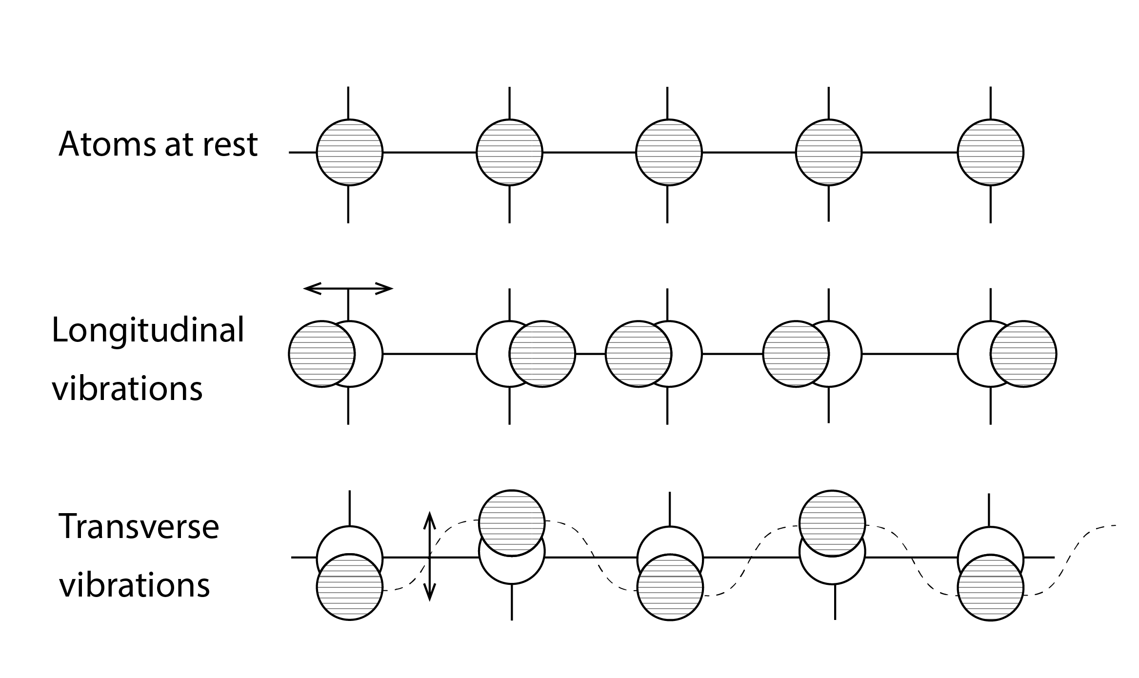
Figure 1: Conduction in non-metallic solids

In the absence of internal heat energy, the atoms or molecules from which the material is comprised would be at rest. In this immobile internal state, the material would have a temperature, in Kelvin, of absolute zero (0K, or -273.15^oC). Heat is always transferred from regions of more excited material or objects, at a higher temperature, to regions or objects of less excited material, at a lower temperature. In other words, and as expressed by The Second Law of Thermodynamics:

Heat cannot spontaneously flow from cold regions to hot regions without external work being performed on the system

When two objects are at the same temperature, there is no transfer of heat between them.

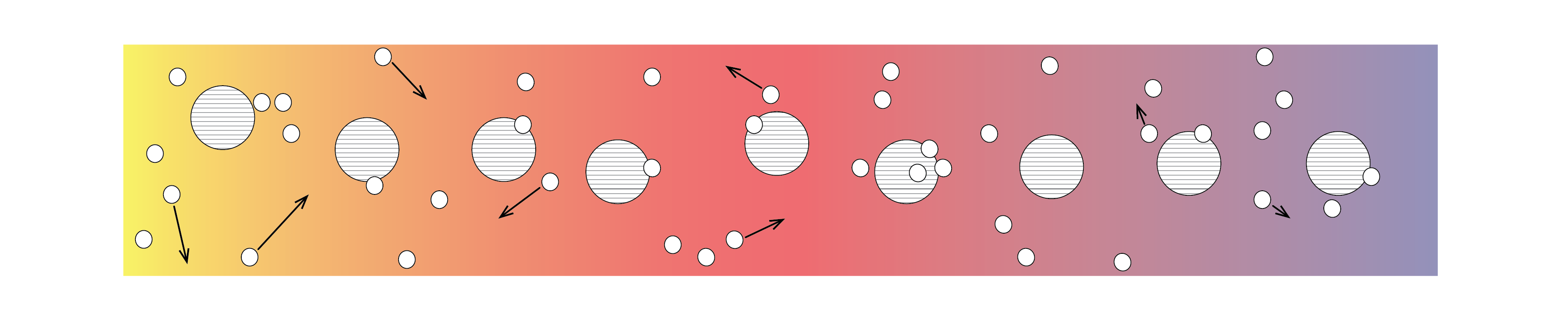
Metallic solids have an abundance of charge carriers, in the form of free electrons. These free electrons also support the transfer of heat by directly transferring their kinetic energy, or indirectly through collisions with other electrons or the atoms from which the metal is comprised (Figure 2).

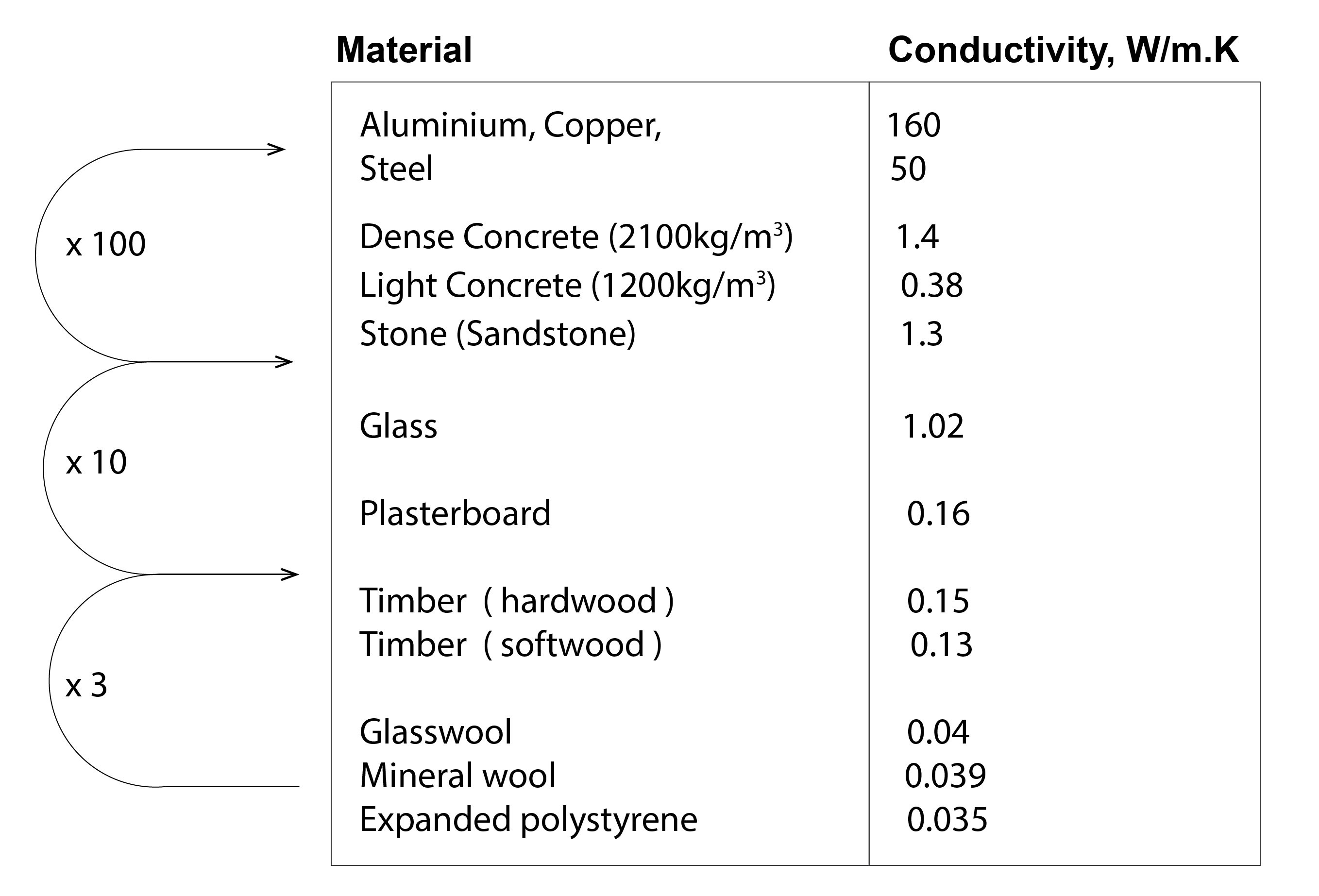
The ability of a material to transfer heat from a warm region (e.g. a warm inside surface of a timber door) to a cold region (e.g. a cool outside surface of a door), is described by its conductivity, which has units of W/(m.K); representing the rate of heat flow (in Watts W, or Joules per Second, J/s) per unit thickness of material and temperature difference across it. The higher the value of a material’s conductivity, the more efficient it is at transferring heat by conduction. The materials towards the bottom of the tabulated figure (Figure 3) below are classed as insulators. They are comprised of malleable (normally fibrous) materials of low density and which accommodate lots of pockets of trapped air. These insulating materials are good at resisting the transfer of heat. Further up, we have hardwood, softwood and plasterboard. These are much more rigid materials that are more effective at transferring heat, but the glass, stone and concrete materials are more effective still, being comprised of much more strongly coupled atoms. They are about 10 times more effective at conducting heat than their timber or plasterboard counterparts. But the metals are around a further 100 times more efficient, owing to the abundance of free electrons – particularly in the case of Copper, which is extensively used as an electrical conductor. Note that steel, commonly used as reinforcement, has a conductivity more than 35 times greater than concrete.

Figure 3: Illustrative conductivities for some common types of constructional material

Heat Conduction

The rate of conductive heat transfer q_cond, in Joules per Second (J/S) or Watts (W), across a material of thickness L (m) and a surface area A, from a warm side at a Temperature T₁ (K) to a cooler side at a Temperature of T₂ (K), is described by Fourier’s Law:

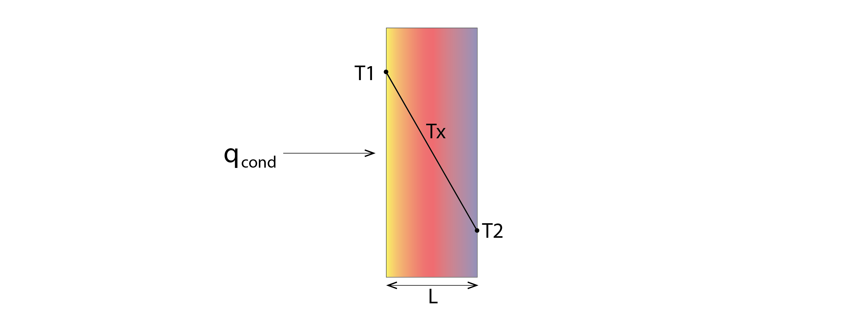
(1) $\begin{equation*} q_{cond} = -k.A \frac {T_2-T_1} {L} \end{equation*}$

Figure 4: 2D section through a hypothetical wall of thickness L

Note that, by convention, when expressing a temperature difference in one dimension (as in Figure 4 above), we subtract the right-hand temperature (T₂) from the left-hand temperature (T₁), but since this would produce a negative heat transfer, we precede our conductivity with a minus sign. Alternatively, we could simply omit this minus and switch the two temperatures, to give the same result (e.g. $q_{cond} = k.A \frac {T_1-T_2} {L}$ ).

Heat Convection

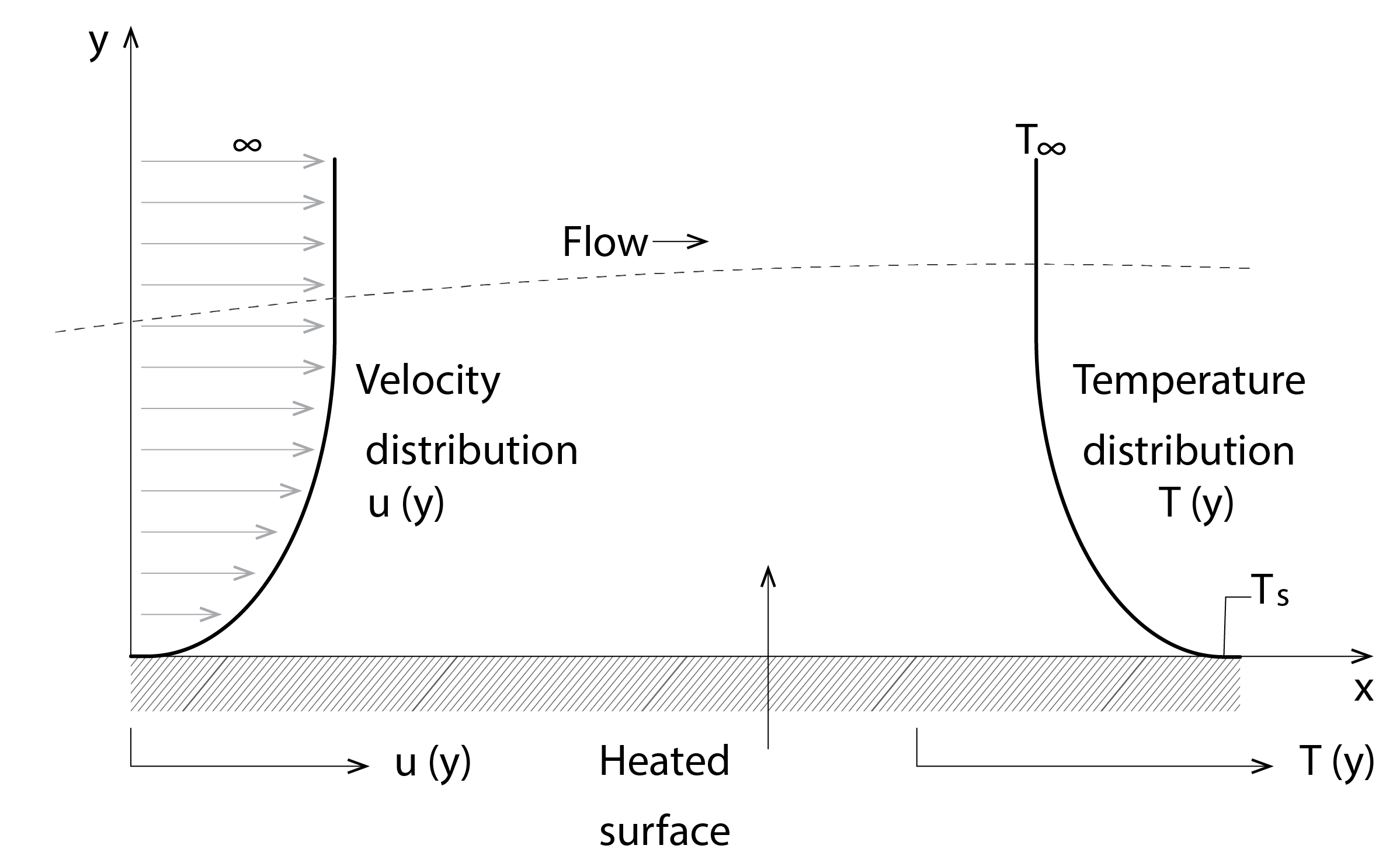
Heat is not only transferred to other regions within a material, it is also transferred from an exposed surface to the adjacent air, by convection, as well as to other adjacent surfaces, by longwave (or infrared) radiation exchange. In the case of convection, when air flows over a heated surface, such as a ground surface that is heated by the absorption of solar energy from the sun (see Figure 5 below), a velocity profile is invoked. The velocity immediately adjacent to the surface is zero^[2], due to viscous shear stresses^[3]. Thereafter, the air behaves somewhat like individual layers slipping over one another, with kinetic energy and heat being transferred between these layers in the direction away from the heated surface due to random molecular diffusion. This continues, as the velocity increases and the temperature decreases, until both profiles asymptote at the free-stream velocity ( $u_\infty$ ) and temperature ( $T_\infty$ , beyond which the rate of change with respect to distance (in direction y) is zero, as indicated in the diagram below). This is referred to as laminar flow.

Figure 5: Velocity and temperature profiles over a flat plate

Consider now a flow of air, at a uniform velocity, arriving at the leading edge of a heated surface (shown lower-left in Figure 6 below), as depicted in the diagram below. Where the flow meets the leading edge, the vertical velocity profile is uniform. Shortly thereafter, a laminar flow regime develops, as in the above scenario, with the velocity increasing from zero at the surface until the free-stream velocity develops at the top of the laminar sublayer. A short distance from the leading edge, a transition develops between this laminar regime in which energy is transferred by random molecular diffusion and a turbulent regime, in which energy is transferred by macroscopic fluid motion, develops. This buffer layer marks the onset of the formation, within the turbulent region, of energetic cells of warm air that rise, detach and circulate in the form of eddies (particles that move in a circular motion). Within this turbulent region, the air temperature and velocity reach their asymptotic values within a very short distance of the buffer layer, as energy is now much more effectively dissipated.

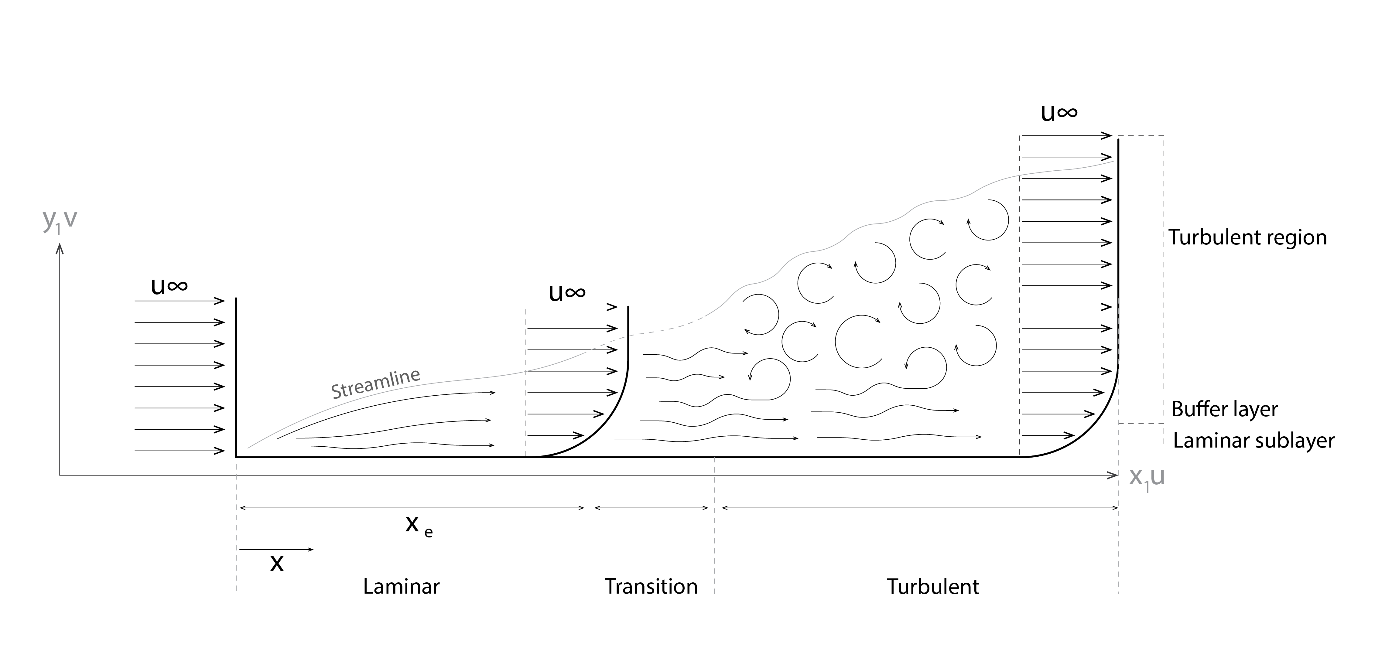
Figure 6: Turbulent and laminar flow regimes

In summary then, whilst velocities are very low (for example where temperature gradients are weak, when background air velocities are particularly low or at the leading edge of a surface) the motion of the air is highly ordered, essentially laminar, with heat transfer being dominated by molecular diffusion. Elsewhere, the airflow tends to be highly irregular. This irregularity increases energy and momentum transfer within this turbulent region. Flows at internal surfaces tend to be more laminar in nature, whereas flows at outdoor surfaces are overwhelmingly turbulent.

We can calculate convective heat transfer q_conv (W) between a surface of area A (m²), at temperature T_s (K) and the air flowing over it at temperature T_a (K) using a convective heat transfer coefficient, h (W/m².K):

(2) $\begin{equation*} q_{conv}=h.A(T_s-T_a) \end{equation*}$

The value of the convective heat transfer coefficient (h) is greater for outside surfaces than it is for inside surfaces. Furthermore, with respect to inside surfaces, ceilings have a lower value than walls, which in turn have a lower value than floors, as heat is progressively more efficiently convected away from the heated surface. According to British Standard (of the European Norm) BS EN 15265, the following are standard values for heat transfer coefficients:

Examples of surface convective heat transfer coefficients
Surface type	Heat transfer coefficient ‘h_c‘ (W/m².K)
Inside floor	5.0
Inside wall	2.5
Inside ceiling	0.7

For the outside case, this coefficient is expressed (in equation form, after McAdams, 1954) as a function of wind speed. The greater the wind speed (v in (m/s)), the more turbulent the air is and thus the convection of heat from the heated surface is more efficient:

(3) $\begin{equation*} h_c=5.6 + 4.0v \end{equation*}$

Heat Radiation

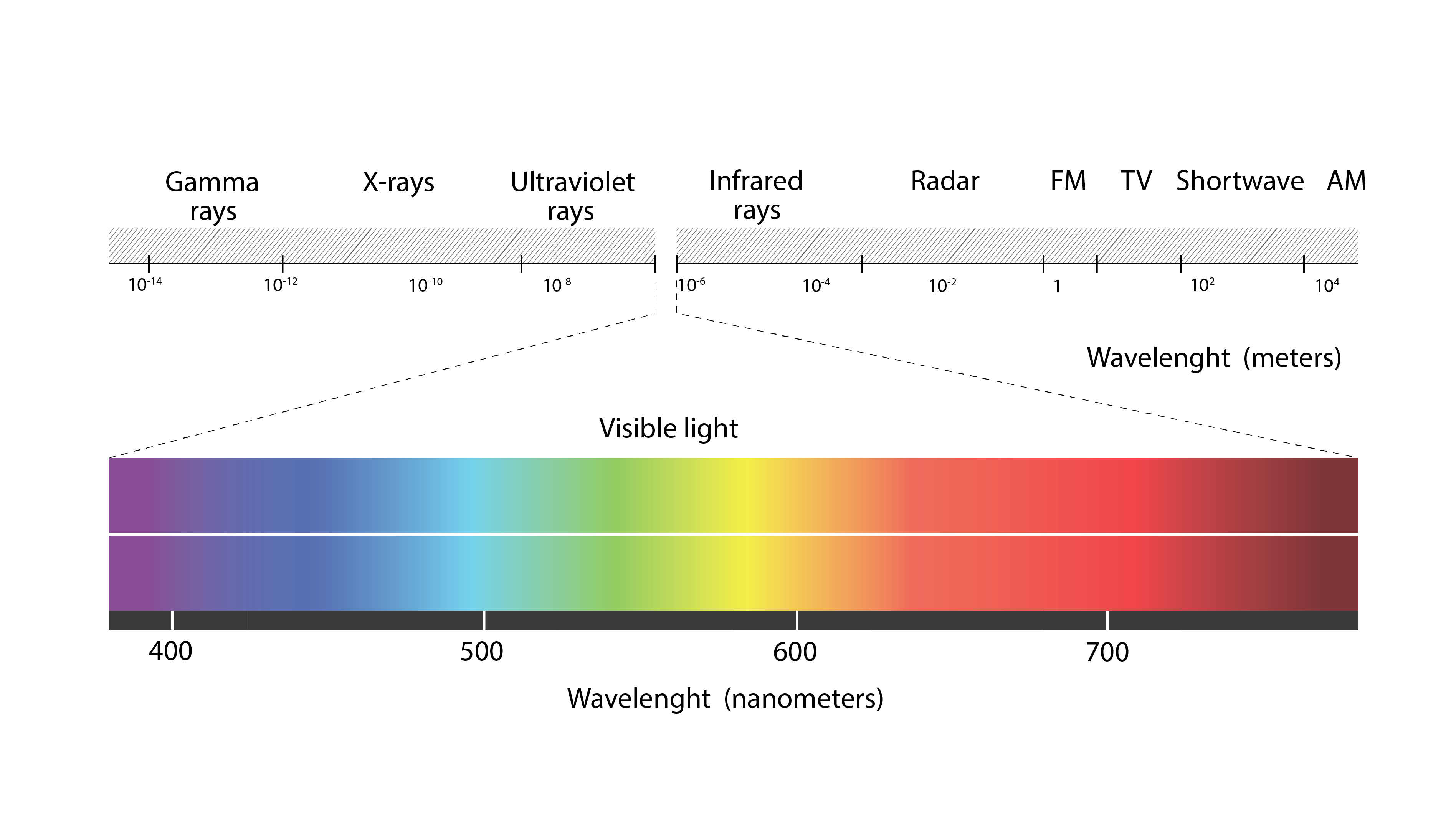
The third and final mode of (sensible) heat transfer is by longwave or infrared radiation exchange from an emitting surface to the receiving surfaces that comprise its bounding external environment (or vice versa). Shown below (Figure 7) is part of the electromagnetic spectrum, which situates the infrared part of the spectrum immediately to the right of the visible part. This part of the spectrum spans a range of 3-4 $\mu m$ to around 100 $\mu m$ . Heat energy is transmitted from this part of the spectrum in the form of electromagnetic waves (or photons, in the complementary particle theory of radiation exchange) to the surrounding receiving surfaces.

Now, the rate of heat (or the heat flux) emitted from a surface $q_{em}\prime (W/m^2)$ depends on the Stephan Boltzmann constant $\sigma$ , which has a value of approximately $5.67 \cdot 10^{-8}, (W/m^2 \cdot K^{-4})$ and the temperature of the emitting surface $T_s$ :

(4) $\begin{equation*} q_{em}\prime=\sigma T_s^4 \end{equation*}$

However, the above expression relates to what we refer to as a ‘black body’, a perfect emitter and absorber of infrared heat (or longwave) radiation. However, surfaces found in nature are not perfectly efficient at emitting and receiving infrared heat radiation. We refer to these surfaces as ‘grey bodies’ and their efficiency is expressed using a surface emissivity $\epsilon$ . Thus, we employ a modified form of the above equation to calculate the heat flux emitted by a real surface:

(5) $\begin{equation*} q_{em}\prime=\epsilon \sigma T_s^4 \end{equation*}$

Reciprocally, the flux absorbed by a surface $q_{abs}\prime$ is the product of the incident radiative heat flux $q_{inc}$ and an absorption coefficient $\alpha$ :

(6) $\begin{equation*} q_{abs}\prime=q_{inc} \alpha \end{equation*}$

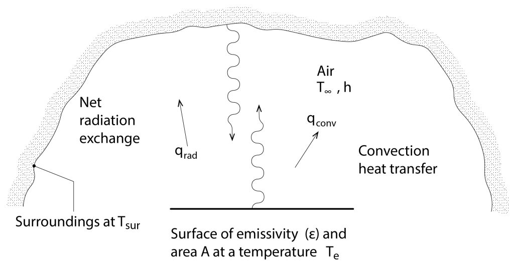
For all practical purposes, we can assume that the emissivity and absorption coefficients are equivalent to one another, so that to calculate the nett radiative heat transfer (W) between our surface of interest s of area A and our surroundings sur (Figure 8), we use the following form of equation, which we refer to as The Stefan-Boltzmann law:

(7) $\begin{equation*} q_{rad}=\epsilon A \sigma (T_s^4 - T_{sur}^4) \end{equation*}$

Figure 8: Radiative heat transfer from a surface to its surrounding environment

The following table (see link for further information) contains examples of measured surface emissivity for some materials that are commonly employed in construction (with the exception of course, of gold). These are arranged in order from surfaces having the lowest emissivity at the top, to those having the highest emissivity at the bottom. From this, it should be immediately apparent that the polished metals have a very low emissivity and are correspondingly very inefficient at emitting heat by radiative exchange. But this inefficiency can be a really useful property. Consider a double-glazed window, comprised of standard glass. Now, the warm inside layer will be heated and will transfer heat by convection to the air in the cavity and it will also efficiently radiate heat to the outside layer, which will also be heated by convection by the air in the cavity. However, if we coat the outside surface of the inside pane with a microscopically thin layer (so that it is invisible to the human eye) of metal, the inner pane will now be much less effective at radiating heat to the outer pane. If we now also fill the cavity with an inert gas like Argon instead of air, then heat will be inefficiently transferred by convection between the inside and the outside pane. This describes a high-performance window, where the outer cold pane is thermally separated from the warm inside pane.

Longwave emissivities for some common exposed types of surface
Material (and surface condition)	Longwave emissivity
Highly polished gold	0.02
Highly polished aluminium	0.05
Heavily oxidised aluminium	0.25
Oxidised copper	0.65
Ceramic earthenware	0.9
Red brick	0.93
Concrete	0.94
Glass	0.95
Paint	0.95

Exposed surfaces of brick, concrete or painted surfaces constructed of other materials will also have a high emissivity, meaning that they can efficiently absorb heat emitted from warm surfaces like radiators, and efficiently emit heat that has been absorbed by solar energy transmitted through a window. This helps to improve the efficiency with which heat is distributed internally.

In a similar vein, metal frames are sometimes bonded to the inside of concrete structures like floors; so that in this case the metal would form an exposed ceiling. Painting this metal surface can transform the metal into an effective radiant absorber, enabling the concrete to more effectively store excess heat from the interior of the room during the day and to discharge this at night.

1.3 Steady state heat transfer

Building on the above principles, this section explains how to calculate the heat flow through multi-layer constructions, how to calculate the surface temperature at the interior and throughout these constructions and how to calculate the energy requirements of rooms as well as whole buildings for space conditioning, with a particular emphasis on heating, and how to take into consideration the effects of thermal bridges.

Fourier’s law and the U-Value

Recall from the above section on heat conduction that the rate of heat transfer from one side of a material to another, $q_{cond}$ , can be determined using Fourier’s Law: $q_{cond} = -k.A \frac {T_2-T_1} {L}$ . Now, if we divide the thickness, $l$ (m), by our conductivity k (W/m.K), then we have a material’s thermal resistance, R (m²K/W): $R=l/k$ . This is convenient because it enables us to add resistances together, rather like an electrical circuit in series, so that we can calculate the heat transfer through materials that are comprised of multiple homogeneous layers, such as walls, roofs and floors, so that for the set of i layers:

(8) $\begin{equation*} \sum_i R = \sum_i (l/k) \end{equation*}$

To this, we can add two further effective layers, representing what we call the film resistance at the indoor and outdoor surfaces. These account for (and are essentially the inverse of) a combination of the relevant convective heat transfer coefficient ( $h_c$ ) and the radiative heat transfer coefficient ( $h_r$ ), so that the surface film resistance $R_s \simeq \frac{1}{h_c + h_r}$ . Thus, and in a similar manner to the calculation of surface convective heat transfer (flux in this case): $q\prime_r = h_r(T_s - T_{sur}) \simeq \epsilon \theta (T_s^4 - T_{sur}^4)$ , so that the radiative heat transfer coefficient ( $W/m^2\cdot K$ ) is a way of linearising^[4] the surface radiative heat flux calculation. The standard values for the internal and external film resistance are as follows:

Surface film resistances
Surface location	Film resistance, $R_s$ ( $m^2 \cdot K/W$ )
Internal surface (i)	0.123
External surface (e)	0.055

With this knowledge, we can now calculate the U-Value of a multi-layer construction – the metric that forms the cornerstone of steady-state heat transfer calculations, heating system sizing calculations and simplified models to predict room and building energy use. Put simply, the U-Value is simply the reciprocal of the total resistance across the entire construction, including the two film resistances:

(9) $\begin{equation*} U = \frac {1}{\sum R} = \frac{1}{R_{si}} + \frac{1}{\sum_i{\frac{l}{k}}} + \frac{1}{R_{so}} \end{equation*}$

Surface temperature

Now that we know how to calculate the U-Value of a multi-layer construction, we can also calculate the surface temperature at any interface through this material (the inside surface, the outside surface, or any contact point between two materials between these exposed surfaces), call this position x. For this we simply need to calculate the cumulative thermal resistance $R_c$ en-route to this point from the inner film in the direction towards the outside:

(10) $\begin{equation*} T_x = T_{ai} - \frac{R_c \Delta T}{\sum R} \end{equation*}$

where the temperature difference ( $\Delta T$ ) between the indoor air (ai) and the outdoor air (ao) $\Delta T = T_{ai} - T_{ao}$ . Put into words, this simply deducts from the indoor air temperature, a fraction of the total temperature difference that is the equivalent to the fraction of the total resistance that is encountered en-route to the position x that we’re interested in.

Often, we’re simply interested in calculating the temperature of the inside surface, whether for indoor thermal comfort assessment or to assess whether there is a risk of surface condensation appearing^[5]. In this case, the calculation appears much more straightforward:

(11) $\begin{equation*} T_{si}=T_{ai}-(U R_{si}\Delta T) \end{equation*}$

From this, we can also calculate a weighted mean of the indoor surface temperature ( $\bar{T}_{si}$ ), which is often a reasonable approximation of the mean indoor radiant temperature ( $T_{mrt}$ ), in other words ( $\bar{T}_{si} \simeq T_{mrt}$ ):

(12) $\begin{equation*} \bar{T_{si}} = \frac{\sum_i({T_{si}}\cdot A_i)}{\sum_i{A_{i}}} \end{equation*}$

Thermal bridges

Thermal bridges are weak links in a building envelope where the thermal integrity is compromised. Figure 9 below presents three categories of thermal bridge: a) relates to a change of material, in this case, the external insulation applied to a wall is interrupted by an uninsulated concrete column, which essentially acts as an uninsulated bridge between the outside and inside boundary conditions of the envelope, b) relates to a geometric discontinuity, in this case at the corner of a room, where the heat flows in two directions rather than a single direction, as is the case away from the corner, c) a combination of the previous two cases: a material change combined with a geometric discontinuity.

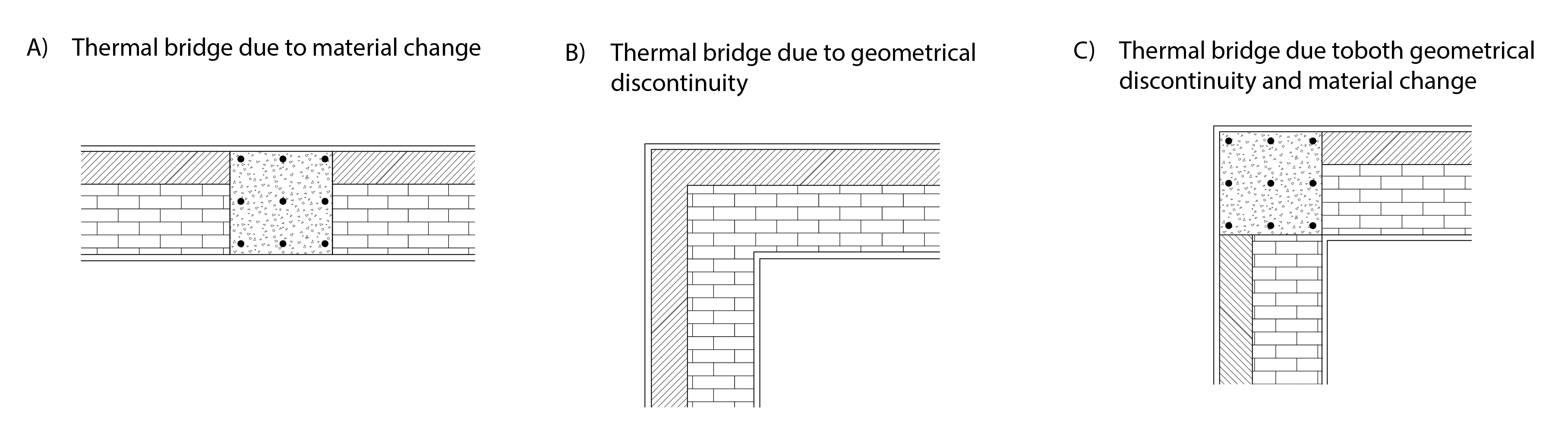
Thermal bridges increase heat loss across the envelope and also reduce (in winter) the inside surface temperature, thus increasing the risk of surface condensation. In the case of geometric discontinuities, this situation can be exacerbated by a lack of air movement, so that surface moisture is not effectively removed and mould can be allowed to grow, compromising occupants’ respiratory health.

Heat loss across thermal bridges is typically calculated using a linear U-Value, $U_{lin}$ ( $W/(m \cdot K)$ ):

(13) $\begin{equation*} q = U_{lin} L (T_{ai}-T_{ao}) \end{equation*}$

where L refers to the length of the thermal bridge, such as a concrete cantilever forming a balcony, which has a linear U-Value of around 0.5 $W/(m \cdot K)$ .

Infiltration and ventilation

In addition to heat loss through the fabric (walls, floor, roof, glazing) of a building envelope, heat is also lost through the flow of air. This can be accidental or deliberate. Accidental airflow is caused by gaps or discontinuities in the building envelope, through which air flows depending upon pressure differences between the interior and the exterior; these being more pronounced under wind weather conditions. This is termed as infiltration, and these kinds of gaps typically occur around the edges of openings such as windows, doors, or at junctions between elements of the envelope, such as between a wall and a floor or a roof. In addition, air can flow through air bricks, open flues and chimneys.

We can calculate the rate of heat loss due to this infiltration ( $q_{inf}$ ), given a corresponding mass flow rate of air $\dot m (kg/s)$ :

(14) $\begin{equation*} q_{inf} = \dot m C_p (T_{ai} - T_{ao}) \end{equation*}$

where $C_p$ refers to the specific heat capacity of air ( $J/kg \cdot K$ ) and the difference in temperature refers to the work that is done in heating the air that infiltrates through the envelope, from its starting temperature $T_{ao}$ to its final temperature $T_{ai}$ . Far more convenient, is to use estimates of infiltration rate, expressed as the number of times per hour $n (h^{-1})$ that the internal volume of air is exchanged with outdoor air. This can then be transformed into an approximate heat loss, using the expression:

(15) $\begin{equation*} q_{inf} \simeq n V (T_{ai} - T_{ao}) / 3 \end{equation*}$

where $nV/3 \simeq \dot m C_p$ for a standard specific heat capacity of air of 1000 $J/kg \cdot K$ and an air density $\rho$ of 1.2 $kg/m^3$ , because:

(16) $\begin{equation*} \dot m C_p = \rho \dot v C_p = \rho n V \frac {1}{3600} C_p = 1.2 \cdot nV \cdot 1000 \frac{1}{3600} = n V \frac {1}{3} \end{equation*}$

Older buildings typically have higher infiltration rates. This is due to the standards of workmanship at the time of construction as well as, indeed in particular, due to deterioration of the building, window and door openings. In a study of 16 post-1930 dwellings in the UK, Pasos et al (2020) measures infiltration rates in the range $0.1 \le n \le 0.5$ , whereas Johnston and Stafford (2016) measured infiltration rates of new dwellings in the range $0.2 \le n \le 0.34$ and Jones et al (2015) estimate infiltration rates throughout the UK housing stock to be in the range $0.02 \le n \le 0.98$ , with the higher values being due to older dwellings.

Sensible, specific and latent heat

Sensible heat refers to the absorption or release of heat energy by a material, due to a change in its temperature. Suppose we have a 5m by 5m concrete floor that is 0.1m thick, so that the volume V of this material is 2.5m³, and we raise its temperature by 5K, from T₁ to T₂. We can calculate the total amount of sensible heat energy Q that would be absorbed in achieving this temperature change thus:

(17) $\begin{equation*} Q = m C_p (T_2 - T_1) = \rho V C_p (T_2 - T_1) \end{equation*}$

where $\rho$ is the density of the material ( $kg/m^3$ ), m is its mass (kg) and $C_p$ is the specific heat capacity – the amount of heat energy required to increase the temperature of 1kg of a substance by 1K $J/kg \cdot K$ . If the density of our concrete is around 2,400 $kg/m^3$ and its specific heat capacity is around 880 $J/kg \cdot K$ , then 26.4MJ of sensible heat energy will have been absorbed in raising its temperature by 5K.

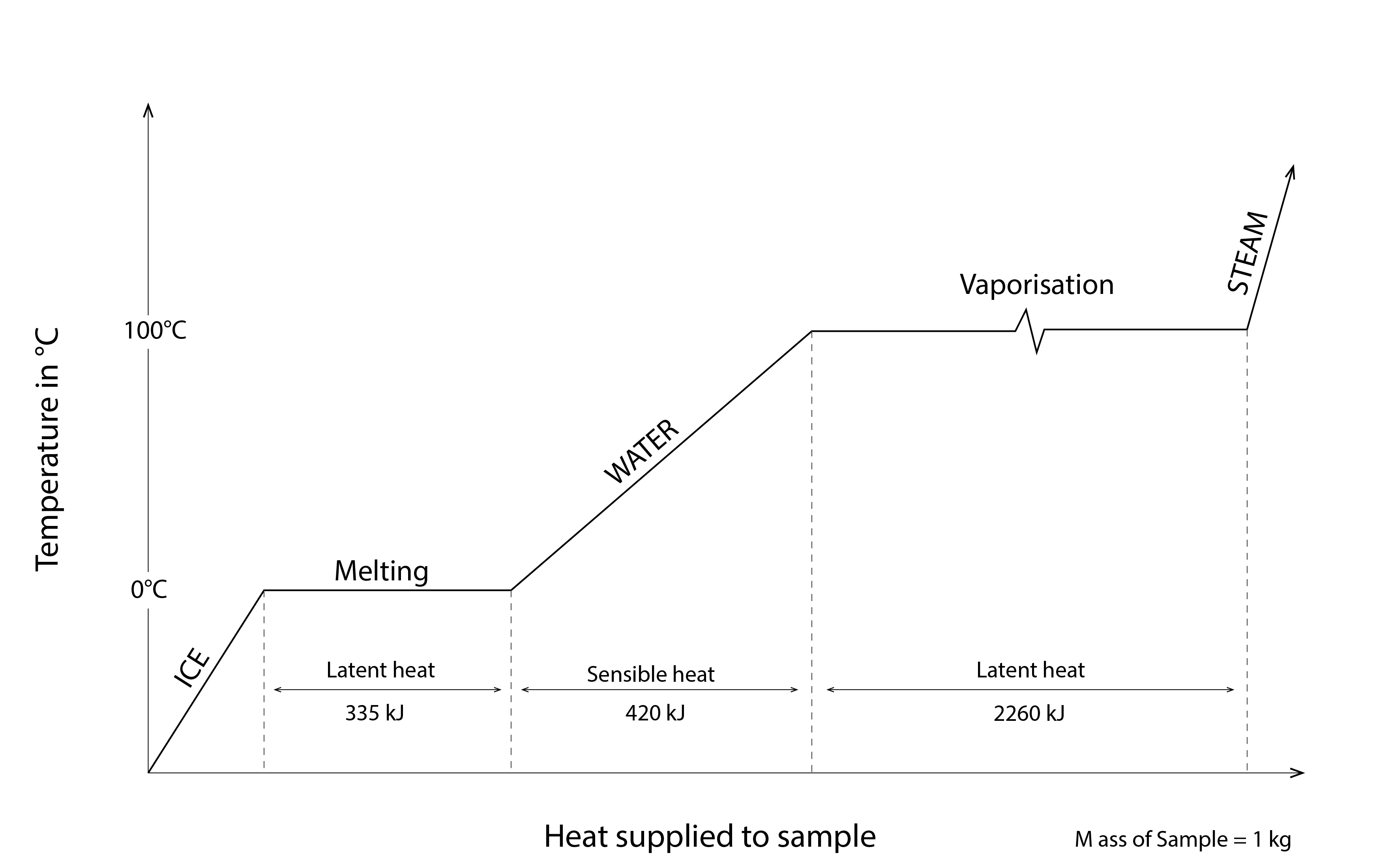
Latent heat L refers to the absorption or release of energy during the change of phase of a material. In the case of water, this could involve a change of phase from a liquid to a solid (or vice versa). This we refer to as the latent heat of fusion $L_f$ . As water freezes to become ice, heat must be removed, the quantity of heat Q being the product of the mass of water m and its latent heat of fusion: $Q = m \cdot L_f$ . Conversely, this same amount of heat must be added as our ice melts from its solid to its liquid phase. Similarly, we must add heat energy to water to support its change of phase from a liquid to a vapour, the amount being determined now by its mass and its latent heat of vaporisation: $Q = m \cdot L_v$ . Once again, this same amount of heat must be removed when this moisture returns from its vapour to its liquid phase. This occurs when moisture condenses on a cool surface, such as a mirror when we take a shower, so that our mirror is slightly heated as vapour condenses on its surface. During changes of phase, the temperature of our substance (e.g. gaseous, liquid or solid water) doesn’t change, even though it is absorbing or discharging heat to accomplish this phase change.

The latent heat of fusion and of vaporisation of water are 0.335 and 2.260 $MJ/kg$ respectively – see Figure 10 below. Thus, if we freeze and subsequently thaw 1 litre of water, having a density of around 1000 $kg/m^3$ , then we must remove and subsequently add 0.335 MJ of heat energy. Similarly, if we evaporate and subsequently condense 1 litre of water, we must successively add and remove 2.260 MJ of heat energy. This is why evaporative cooling can be such an effective passive cooling strategy – the latent heat of vaporisation of water is really high!

Room heat loss and energy balance

Now that we know how to calculate the U-Value of a multi-layer construction, we can also calculate the corresponding rate of heat loss q ( $W$ or $J/s$ ):

(18) $\begin{equation*} q = U \cdot A (T_{ai} - T_{ao}) \end{equation*}$

By extension, we can also calculate the total rate of heat loss through all of the i multi-layer constructions from which a room is comprised, as well as that due to infiltration:

(19) $\begin{equation*} q = ( \sum_i (U \cdot A) + n \cdot V / 3) (T_{ai} - T_{ao}) \end{equation*}$

Heating systems

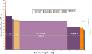
Shown below (Figure 11) is a histogram of the distribution of heating systems throughout the UK housing stock. For each of the main types of system identified by the white labels, the x-axis indicates the total floor area of UK housing that adopts this system, whereas the y-axis identifies the average energy use, normalised by floor area. From this, it is clear that gas central heating systems are dominant. These are systems where a central gas-fired boiler heats water that is distributed by pipes to a network of radiators in the rooms of the house. Interestingly, around 80% of the heat from these radiators is transferred by convection, the remainder by radiation. Gas-back boilers, combi boilers and oil-fired boilers are essentially variants of this type of gas-fired central heating. The average efficiency $\eta$ of older boilers can be as low as 65% and that of new boilers can be as high as 95% so that (with efficiency expressed as a fraction) $0.65 \le \eta \le 0.95$ . A number of houses and flats are heated by direct electric heaters; some of these being instantaneous convector heaters, some being storage heaters, which use off-peak (nighttime) electricity to heat high thermal capacity bricks which later transfer this heat to the room by natural convection. These systems are essentially perfectly efficient, as all of the electrical energy degrades to heat.

More recently, we have started to witness the introduction of heat pumps. The functioning of heat pumps is almost identical to that of a standard refrigerator, which is another example of a hydraulic network, this time comprised of an evaporator (inside the refrigerator), a compressor, a condenser (the painted pipes at the rear of the radiator) and an expansion valve. Within this system, a refrigerant is circulated. This is just a fluid that has a low boiling point. Within the evaporator, the refrigerant changes phase from liquid to gas and in so doing the energy required for this change of state (the latent heat of vaporisation) is provided by the interior of the fridge thus cooling it down. The refrigerant’s pressure is then increased by the compressor before it passes to the condenser, where it now changes phase from a gas to a liquid, transferring its latent heat to the air at the back of the fridge. The refrigerant then passes through an expansion valve where its pressure is reduced, before once again passing to the evaporator.

Heat pumps can be very efficient, with this efficiency depending upon the temperature of the environment that the evaporator and condenser are in contact with. In heating mode, the evaporator is exposed to the air (air-source) or the ground (ground-source), whereas the condenser is essentially the network of pipes and radiators. Ground-source heat pumps are more efficient than air-source heat pumps, because the ground (from which heat is transferred via a horizontal or a vertical circuit) is usually warmer than the air. The efficiency of heat pumps is expressed as a coefficient of performance, or CoP (sometimes called a seasonal performance factor, or SPF). Air-source heat pumps have a CoP of: $2.5 \le CoP \le 3.5$ , whereas ground-source heat pumps can have a CoP of $3.5 \le CoP \le 6.5$ . This means that, for each unit of electrical energy that is used by the heat pump, as much as 6,5 units of heat can be provided!

Energy use estimation

In the solution to problem 3 (P3) in section 1.5 below, we calculate a total room conductance C_r( $W/K$ ), where $C_r = (\sum_i (U \cdot A) + n \cdot V / 3)$ . By extension, we can also calculate a total building conductance, call this C_b, by simple addition of the individual room conductances, so that $C_b=\sum_r C_r$ . From this we can estimate the annual amount of energy that is required to heat the building, $Q_{heat}$ ( $kWh/m^2$ ), so long as we know the heating degree days (HDD) for the corresponding location and the efficiency of the heating system $\eta$ :

(20) $\begin{equation*} Q_{heat} = \frac{24 \cdot HDD \cdot C_b}{1000 \cdot \eta \cdot A_F} \end{equation*}$

where $A_F$ is the treated floor area (the floor area of the building that is heated). This is a way of normalising the calculation so that we can conveniently compare the calculated energy use with benchmarks or other buildings, for which the energy use has also been normalised.

But what are these heating degree days (HDD)? All glazed buildings transmit some energy from the sun. They also normally benefit from what we call casual heat gains. This is the emission of heat from lights, electrical devices (e.g. TVs, laptops), cooking equipment and even people (as each person emits around 90W of heat), mainly by convection and radiation. Because of these solar and casual heat gains, we don’t need to activate a heating system to heat a building so long as the daily average outdoor air temperature is at or above what we refer to as a balance point temperature. In the UK, we normally assume that this is around 15.5^oC, but the actual value depends on the characteristics of the building that we’re studying. So, if the mean daily outdoor air temperature is 15.5^oC then we assume that the solar and casual heat gains are sufficient to raise the mean indoor air temperature to a comfortable level, say 20^oC. If the mean daily outdoor air temperature is above 15.5^oC, then the mean indoor air temperature should likewise be above 20^oC. However, if the mean daily outdoor air temperature is below 15.5^oC, then heat energy will need to be delivered from the heating system to achieve our 20^oC comfort temperature.

By way of example, if the mean daily outdoor air temperature is 12.5^oC on a given day, we will have accumulated 3 HDD. By multiplying this by 24, we convert this into heating degree-hours ( $K \cdot h$ ). By multiplying this by our conductance ( $W/K$ ) we now have an energy demand ( $W \cdot h$ ), which we in turn convert to $kWh$ when we divide this value by 1000. Finally, by dividing by our heating system efficiency we convert an energy demand into energy use and by now dividing by floor area we then finally normalise our result for comparison purposes ( $kWh/m^2$ ).

1.4 Transient heat transfer

The materials from which buildings are constructed both conduct and store heat. Steady state heat transfer calculations ignore this storage of heat. Ignoring this can have important consequences for indoor conditions, the power demands of heating (and cooling) systems to meet requirements for indoor comfort and the use of energy in delivering these comfort conditions. In this section, we examine how heat storage influences the transmission of heat and how this can be accounted for in energy calculations.

Heat storage

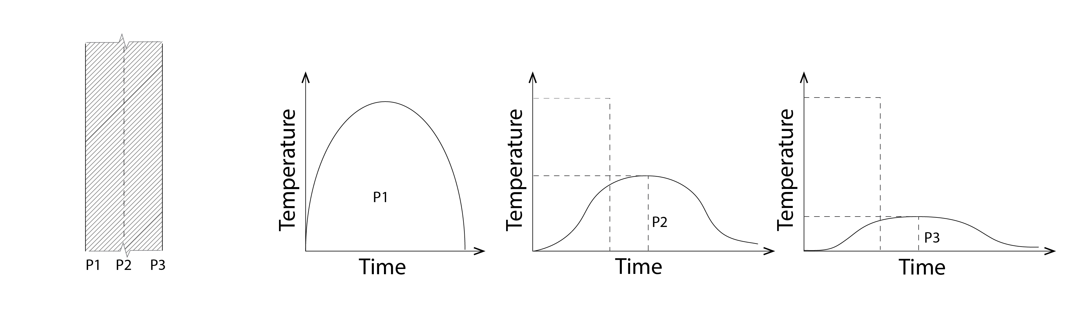
Consider a daytime temperature signal, incident at the outside face of a wall, at position P1 in the image below (Figure 12). This temperature increases whilst the intensity of solar energy increases and then decreases so that the temperature signal (the evolution of temperature with respect to time) at this position resembles half of a sine wave. This temperature signal arrives at position P2 with both a delay and a reduced amplitude with respect to that at P1, so that the peak temperature is both lower and occurs later than that at P1; likewise with respect to P3. This phase difference (the delay) and reduction in amplitude (the lower peak temperature) has significant implications for indoor comfort and the demand for energy to meet occupants’ comfort requirements.

Heat diffusion

Consider an infinitesimally small differential control volume (Figure 13)^[6] of homogeneous material, $dx \cdot dy \cdot dz$ . In what follows we will focus exclusively on the transfer of heat in the x-direction.

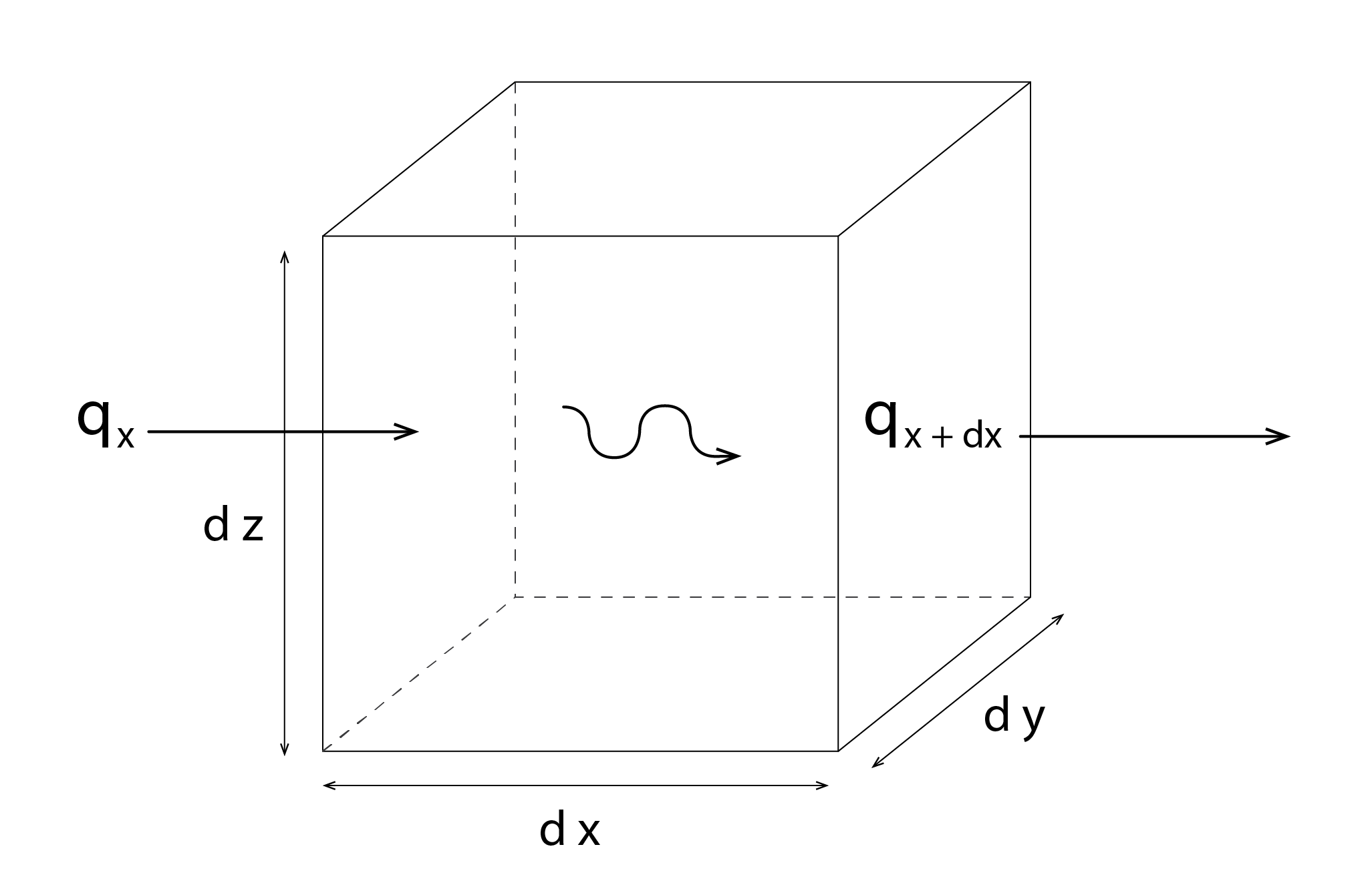
Figure 13: An infinitesimal control volume

The x component of the heat transfer rate leaving our control volume ( $\dot E_{out}$ ) at x+dx is equal to the rate of this component entering our control volume at x ( $\dot E_{in}$ ) plus the amount by which it changes with respect to x times dx:

(21) $\begin{equation*} q_{x+dx}=q_x+\frac{\partial{q_x}}{\partial{x}}dx \end{equation*}$

within this material, there may also be an energy source associated with a rate of thermal energy generation ( $\dot E_{g}$ ):

(22) $\begin{equation*} \dot E_g = \dot q \; dx dy dz \end{equation*}$

Where $\dot q$ is equal to the rate at which energy is generated per unit volume of our material ( $W/m^3$ ). In addition, changes in the amount of thermal energy stored within the material in our control volume may also take place. The rate of energy storage in our control volume is:

(23) $\begin{equation*} \dot E_{st} = \rho C_p \frac{\partial{T}}{\partial{t}} dx dy dz \end{equation*}$

where $\rho C_p {\partial{T}}/{\partial{t}}$ is the time rate of change of internal thermal energy of the material per unit volume.

We can combine these terms in the form of an energy balance, such that:

(24) $\begin{equation*} \dot E_{in} + \dot E_g - \dot E_{out} = \dot E_{st} \end{equation*}$

or in full:

(25) $\begin{equation*} q_x + q_y + q_z + \dot q dx dy dz - q_{x + dx} - q_{y + dy} - q_{z + dz} = \end{equation*}$

$\rho C_p \frac{\partial{T}}{\partial{t}} dx dy dz$

If we substitute into this our equation for $q_{x+dx}$ (and $q_{y+dy}$ and $q_{z+dz}$ ) – equation (21), so that our terms for $q_x$ , $q_y$ , $q_z$ cancel, we have:

(26) $\begin{equation*} -\frac{\partial{q_x}}{\partial{x}}dx -\frac{\partial{q_y}}{\partial{y}}dy -\frac{\partial{q_z}}{\partial{z}}dz + \dot q dx dy dz = \end{equation*}$

$\rho C_p \frac{\partial{T}}{\partial{t}} dx dy dz$

From Fourier’s law, the heat conduction rate in direction x ( $q_x$ ) is:

(27) $\begin{equation*} q_x = -k \; dydz \frac{\partial{T}}{\partial{x}} \end{equation*}$

Substituting this into equation 26 and dividing by the dimensions of our control volume gives the heat diffusion equation with which we can determine the temperature distribution (Tx,y,z) as a function of time:

(28) $\begin{equation*} \frac{\partial{}}{\partial{x}} (k \frac{\partial{T}}{\partial{x}}) \frac{\partial{}}{\partial{y}} (k \frac{\partial{T}}{\partial{y}}) \frac{\partial{}}{\partial{z}} (k \frac{\partial{T}}{\partial{z}}) + \dot q = \end{equation*}$

$\rho C_p \frac{\partial{T}}{\partial{t}} dx dy dz$

If the conductivity is constant throughout our material, this simplifies to:

(29) $\begin{equation*} \frac{\partial^2{T}}{\partial{x^2}} + \frac{\partial^2{T}}{\partial{y^2}} + \frac{\partial^2{T}}{\partial{z^2}} + \frac{\dot q}{k} = \frac{1}{\alpha} \frac{\partial{T}}{\partial{t}} \end{equation*}$

where $\alpha = \frac{k}{\rho C_p}$ is the thermal diffusivity of our material: the ratio of the material’s ability to conduct heat relative to its ability to store heat.

Finally, for heat flow in one ( $x$ ) direction only and with no internal energy generation:

(30) $\begin{equation*} \frac{\partial^2{T}}{\partial{x^2}} = \frac{1}{\alpha} \frac{\partial{T}}{\partial{t}} \end{equation*}$

This is the form of the equation that is typically solved to calculate the flow of heat through multilayer constructions in standard building energy simulation programs.

Principles of energy simulation

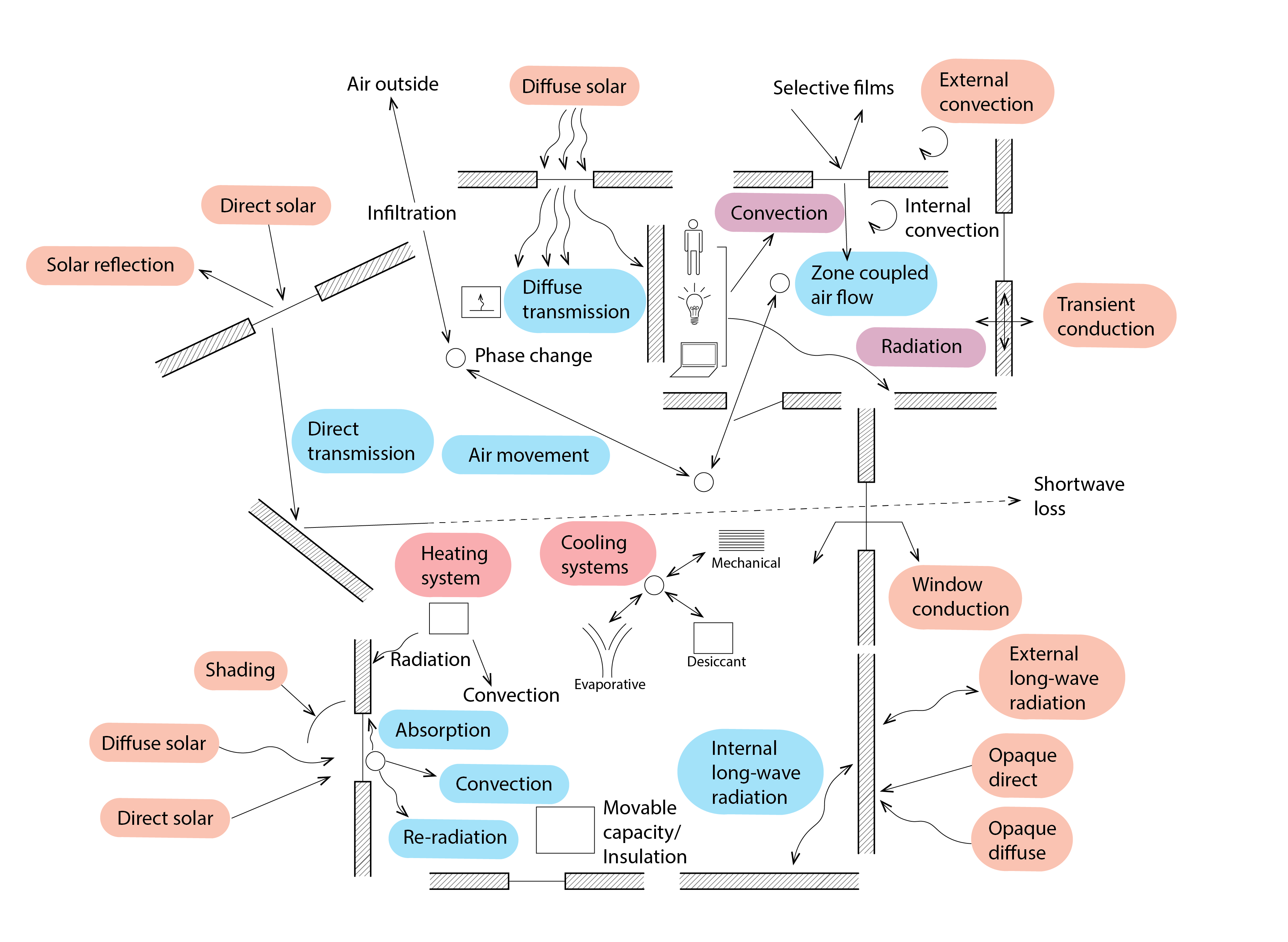
The above equation for the diffusion of heat in one direction for a material of uniform conductivity and with no internal energy generation lies at the core of most dynamic building energy simulation programs, such as EnergyPlus or IES-VE’s Apache program. Unsurprisingly however, there is somewhat more to these programs. As the diagram below (Figure 14) suggests, we must determine the position of the sun relative to the surface from which our building is comprised, in order to calculate the amount of direct solar radiation from the sun that is incident on and perhaps transmitted by (in the case of glazing) these surfaces. In a similar manner, we must also represent how diffuse solar energy is distributed throughout the sky vault, and calculate the corresponding amount of solar energy from the sky that is incident on our building surfaces. This direct and diffuse solar radiation may also be modified by fixed or moveable shading elements. In a similar manner, we must also calculate the amount of net infrared longwave radiation that is emitted from our building’s surfaces. Within the building, we also need to consider the time profile by which casual heat gains (from lights, people and appliances) are emitted, and the proportion of these gains that is emitted by convection and radiation. We also need to consider the flows of air between our building and the outdoor environment due to infiltration as well as deliberate ventilation. Finally, heating, ventilating and air-conditioning (HVAC) equipment may be activated to achieve acceptable levels of comfort for our building’s inhabitants.

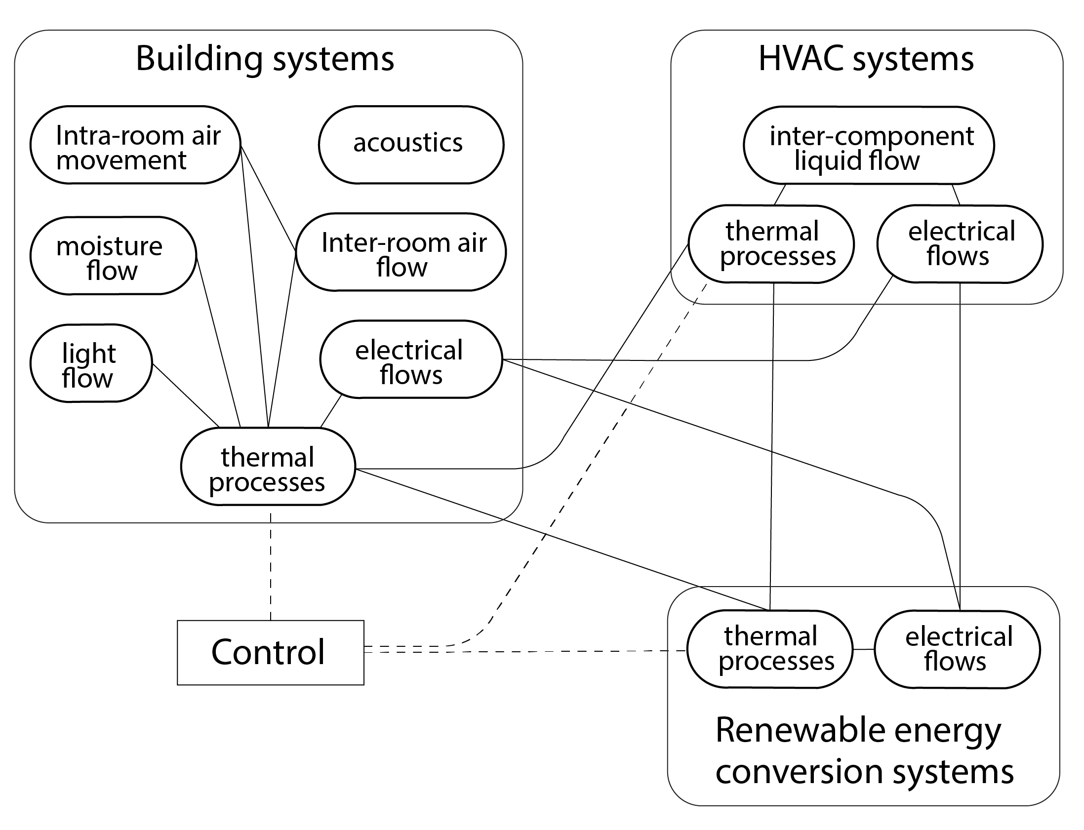
Figure 14: Heat transmission pathways in buildings (adapted from Clarke, 2001). Processes shown in orange correspond to external surface energy exchanges; those in blue correspond to internal surface exchanges; those in red to internal energy systems; those in purple to emission from internal heat gains.

In addition to these quite complex energy flow pathways, the more sophisticated simulation programs are capable of simulating additional performance domains (e.g. moisture, light, acoustics), some of them simultaneously. This might involve the use of dedicated programs to dynamically simulate flows of air within the building and between the building and the outdoor environment and how this is controlled through ventilation openings. Sophisticated models may also be called upon to calculate the distribution of daylight within the interior and how artificial lighting systems react to this availability of daylight. Sophisticated models of the functioning of HVAC equipment may also be called upon, and these may even be coupled with models of renewable energy technologies to meet the needs of this equipment. These and other performance domains are represented in Figure 15 below.

Figure 15: Alternative domains of energy simulation (adapted from Clarke, 2001)

Sophisticated multi-domain simulation programs such as this are increasingly employed by both architecture and engineering companies to support the design and optimisation of the performance of complex buildings, typically within an urban context, which itself influences the local microclimate with corresponding impacts on building performance. These mechanisms and their effects are discussed in the final chapter of this book.

1.5 Questions and worked examples

This section contains a series of worked examples or problems (P) and their solutions (S), as well as a series of written questions (Q) and their written answers (A).

P1) Let’s calculate the U-Value for a wall that is comprised of a 100mm thick layer of stone that has a conductivity of 1.3 $W/m \cdot K$ , a 50mm layer of mineral wool insulation with a conductivity of 0.039 $W/m \cdot K$ and a 100mm thick inside layer of lightweight concrete, with a conductivity of 0.38 $W/m \cdot K$ .

P2) Calculate the inside surface temperature of the wall from P1, given that the indoor temperature is 20^oC and the outdoor temperature is 0^oC.

P3) A single-roomed office building is 5m wide, 5m deep and 3m high. Each of the facades has a U-Value of 0.556, as in the solution to P1. They also each have a glazing ratio of 20%, so that 80% of the wall area is opaque and 20% is glazed. This is single-glazed and 6mm thick, where the glass has a conductivity of 1.02 $W/m \cdot K$ . Assuming that the roof has a U-Value of 0.6 $W/m^2 \cdot K$ , that the floor has a U-Value of 0.45 $W/m^2 \cdot K$ , that the room infiltration rate is 1 $h^{-1}$ and that the indoor and outdoor air temperatures are 20^oC and 0^oC respectively (as in P2), let’s calculate the total room heat loss.

P4) Based on the total annual heating degree days for Sheffield of 2350 and a heating system efficiency of 0.85, calculate the annual heating energy use for the simple office described in P3.

S1) For this kind of exercise, it is useful to perform a spreadsheet calculation of the total thermal resistance, in the form of a table which should look like this:

Material	Thickness, m	Conductivity, $W/m \cdot K$	Resistance, $m^2 \cdot K/W$
Inside film	—	—	0.055
Stone	0.1	1.3	0.077
Mineral wool insulation	0.05	0.039	1.282
Lightweight concrete	0.1	0.38	0.263
Outside film	—	—	0.123
Total thermal resistance			1.800

Since we know that the U-Value is simply the reciprocal of this total thermal resistance, we can now straightforwardly calculate it: $U = \frac {1}{\sum R} = \frac{1}{1.8} = 0.556 (W/m^2 \cdot K)$ .

S2) As we saw earlier, we can calculate the surface temperature using the following equation: $T_{si}=T_{ai}-(U R_{si}\Delta T)$ . So, inputting our values to this equation, we have:

$T_{si}=20-(0.556 \cdot 0.123 \cdot 20)$

$T_{si}=18.63^oC$

S3) Firstly, we need to calculate the U-Value of the single glazing:

Material	Thickness, m	Conductivity, $W/m \cdot K$	Resistance, $m^2 \cdot K/W$
Inside film	—	—	0.055
Glass	0.006	1.02	0.006
Outside film	—	—	0.123
Total thermal resistance			0.184
U-Value			5.438 ( $W/m^2 \cdot K$ )

We can now calculate the total room heat loss:

	Area, $m^2$	U-Value, $W/{m^2 \cdot K}$	Conductance, $W/K$	Heat flow rate, $W$
Wall	48	0.556	26.66	553
Floor	25	0.450	11.25	225
Roof	25	0.600	15.00	300
Glass	12	5.438	65.26	1305
Infiltration			25.00	500
Total	—	—	143.17	2863

Thus, a heating system with a capacity of almost 3kW would be needed to heat this small one-room office building.

S4) As noted earlier, we can calculate our energy use using the following equation: $Q_{heat} = \frac{24 \cdot HDD \cdot C}{1000 \cdot \eta \cdot A_F}$ . Inputting the values into this equation we have:

$Q_{heat} = \frac{24 \cdot 2350 \cdot 143}{1000 \cdot 0.85 \cdot 25}$

$Q_{heat} =380 (kWh/m^2)$

Q1) The British love their tea, for which they regularly heat water using an electric kettle. The body of these kettles is normally made from polished metal (e.g. chrome). Why?

Q2) In the example modelled in P2 and P4 above, the rate of heat loss and the total annual energy use for heating are estimated. This energy use is particularly high. Where do you think there is good potential for reducing this energy use?

A1) Polished metal surfaces have a low emissivity, so they are less efficient at transfer heat by longwave radiative exchange. This means that the water warms quicker and the heat is retained for longer.

A2) The first and most obvious strategy would be to improve the quality of the glazing. For example, using double glazing with a low emissivity coating and perhaps also Argon filled. This would reduce the U-Value to around 2 ( $W/{m^2 \cdot K})$ ). The degree of thermal insulation in the roof, floor and walls could also be substantially improved, say to 0.3, 0.3 and 0.25 $W/{m^2 \cdot K})$ respectively, and the infiltration rate could be substantially reduced, say to 0.25 ( $h^{-1}$ ). Finally, the heating system efficiency could be improved by replacing what is probably an older gas boiler with a heat pump, having an average seasonal performance factor of around 2.5. If all of these changes were implemented, then the energy use would be reduced to just 52 $kWh/m^2$ .

References

BS EN 15265: Energy performance of buildings – Calculation of energy needs for space heating and cooling using dynamic methods – General criteria and validation procedures, 2007.

Clarke, J.A. (2001) Energy simulation in building design (2nd Ed): Butterworth-Heinemann.

Johnston, D., Stafford, A. (2016) Estimating the background ventilation rates in new-build UK dwellings – Is n50/20 appropriate?, Indoor and Built Environment, 26:4, 2016.

Jones et al (2015), Assessing uncertainty in housing stock infiltration rates and associated heat loss: English and UK case studies, Building and Environment, Volume 92, October 2015, Pages 644-656.

Pasos et al (2020), Estimation of the infiltration rate of UK homes with the divide-by-20 rule and its comparison with site measurements, Building and Environment 185 (2020) 107275

McAdams, W.H. (1954), Heat Transmission, McGraw-Hill, 1954.

1 Heat, temperature and thermal energy

1.1 Introduction

1.2 Heat and temperature

Heat Conduction

Heat Convection

Heat Radiation

1.3 Steady state heat transfer

Fourier’s law and the U-Value

Surface temperature

Thermal bridges

Infiltration and ventilation

Sensible, specific and latent heat

Heating systems

Energy use estimation

1.4 Transient heat transfer

Heat storage

Heat diffusion

Principles of energy simulation

1.5 Questions and worked examples

References

Further reading

Licence

Share This Book