
6 Daylight in architecture
physical principles and technologies
The aesthetics of the interior of buildings depends fundamentally on the quality with which they are lit, or illuminated, both naturally and artificially. This quality of illumination is influenced by the magnitude of light, how it is distributed spatially and also how it is distributed spectrally, in the region of the electromagnetic spectrum that the human eye has evolved to be sensitive to. This spectral distribution depends upon the source of illumination and how the light emitted from this source is in turn influenced by the objects through which it is transmitted and from which it is reflected, as well as the perception of the human observer. This visual perception is the ability to interpret the surrounding environment through photopic vision (daytime vision), colour vision, scotopic vision (night vision), and mesopic vision (twilight vision), using light in the visible spectrum. That is, in the range of 380 to 780 nm.
The transmission and reflection of light can be controlled using both static and dynamic technologies, to avoid glare, and to enhance daylight penetration and the spatial uniformity of the transmitted light. Through artificial lighting controls, this can then displace the need for artificial lighting, with corresponding energy savings and reductions in Carbon Dioxide emissions.
6.1 Visual perception: light and the human eye
In humans, light enters the eye through the cornea and is focused by the lens onto the retina, a light-sensitive membrane at the back of the eye, which converts light into neuronal signals using photoreceptive cells known as rods and cones. These cells detect the photons of incident light and respond by producing neural impulses that are transmitted by the optic nerve to the brain.
The total luminous flux  (defined in table 1 below) in lumens [lm] in a source of light is given by the following equation:
(1) 
where  is the peak luminous efficacy (683 lm/W) of the eye at a wavelength of 555nm,
  represents the spectral variation of this efficacy, normalised to a value of unity at a wavelength
  of 555nm (see the image below) and
  is the spectral radiant flux [W/nm].
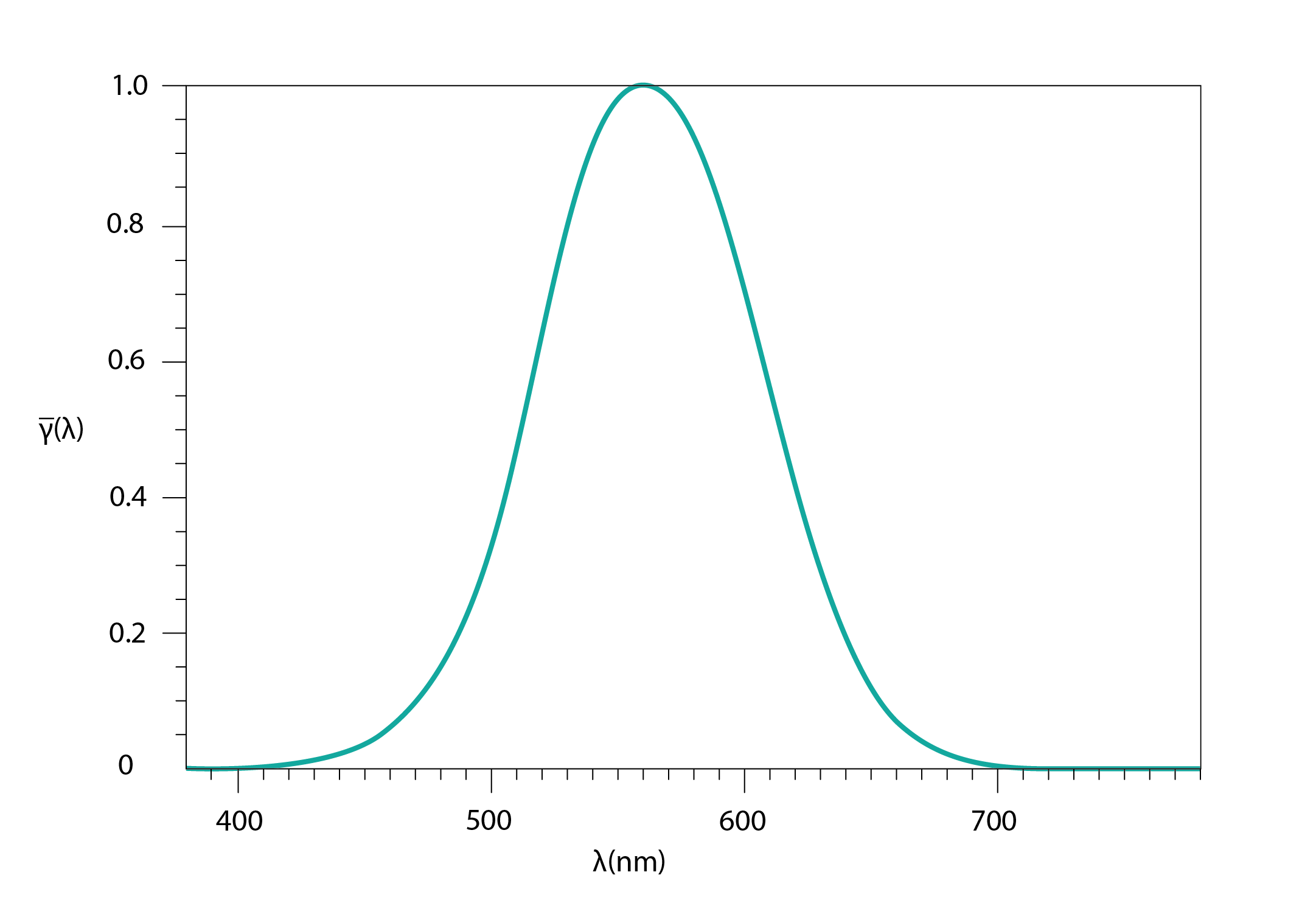
In low light levels, in which only the rod cells are active, the luminosity function is skewed towards lower wavelengths, so that the peak efficacy occurs at around 407nm. This means that the eye is less able to discriminate between colours at lower levels of spectral radiant flux (essentially, at lower light intensities).
6.2 Some principles of optics: reflection, transmission and refraction
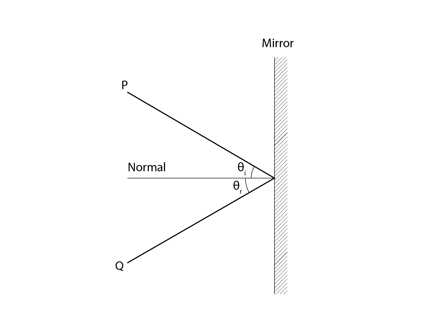
When light is incident at an angle  on a surface like a mirror, this light is specularly reflected in the opposite direction at an angle
  . When we gaze at a mirror we see a perfect reflected image of ourselves.
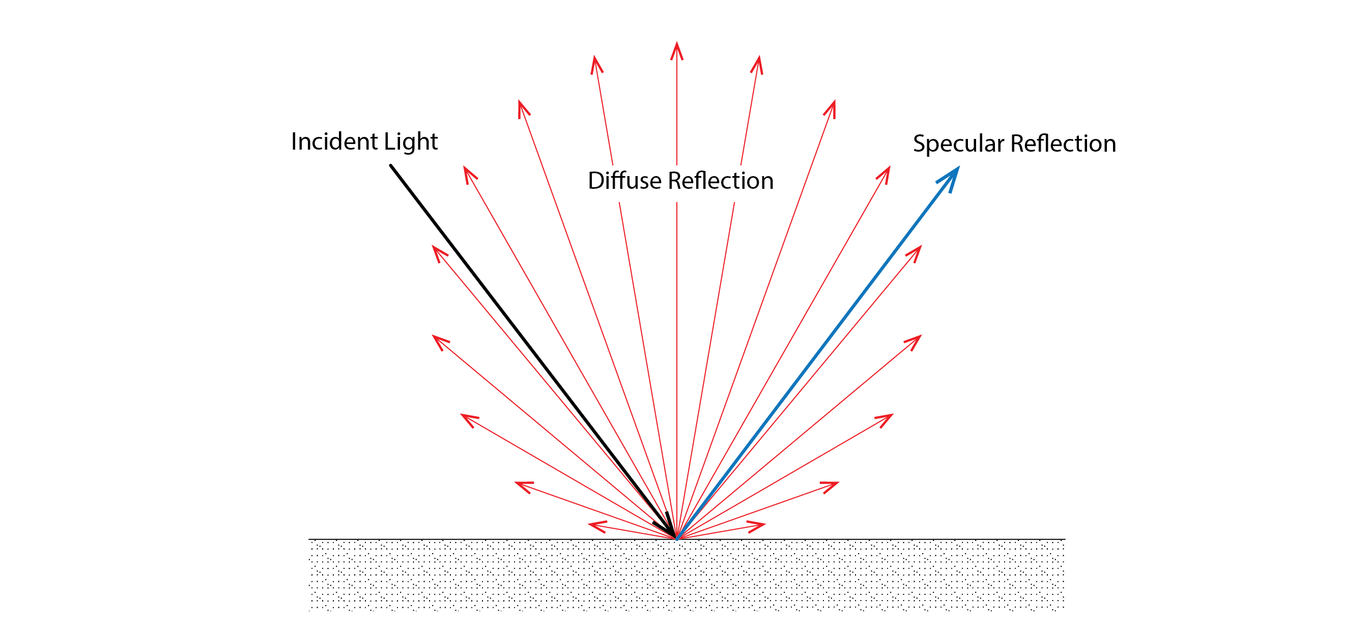
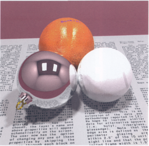
Most surfaces that we find within and outside our buildings don’t reflect light in this kind of specular manner. They contain imperfections in the texture of their surfaces which act to diffuse the reflection of light. We refer to these diffusely reflecting surfaces as Lambertian reflectors. The image below contrasts the behaviour of specular and diffuse reflectors. In the specular case, we see the expected mirrored reflection, whereas in the case of a diffuse reflector, we see that light is emitted throughout a hemisphere from the reflecting surface, the intensity of this reflected light reducing with the cosine of the angle of reflection, so that more luminous energy is emitted in the direction of the surface normal (or perpendicular) and progressively less towards an angle parallel to this surface.
This is a useful observation, because it means that if we can measure the illuminance E incident on a surface [lm/m2] as well as the brightness or luminance L (lm/(m2.Sr)) of this surface, we can calculate its reflectance,  , by re-arranging the relation
  :
:
(2) 
This is because if we integrate the emission of light about a hemisphere of a reflecting surface we have that:  . Thus the luminance of a Lambertian surface is the product of the incident illuminance and the surface’s reflectance, divided by the result of this double integral
  .
.
At this point it is useful to clarify some terms, their units and their definitions:
| Term | Unit | Definition |
| Luminance | lm/(m2.Sr) or Cd/m2 | The brightness of a point source of light or a point on a surface that is receiving light |
| Luminous Flux | lm | 1 lm corresponds to the luminous flux emitted within one Sr by a point source of light of one Cd. A point source emitting a uniform intensity of 1 Cd in all directions emits a total flux of 4 lm |
| Illuminance | lm/m2 or lux | Luminous flux reaching a surface per unit area |
| Luminous efficacy | lm/W | The ratio of luminous and radiant fluxes – based on a CIE standard human eye response |
| Steradian | Sr | The solid angle at the centre of a sphere that cuts an area on the surface of a sphere equal in size to the radius squared. There are 4 Sr in a sphere |
| Candela | Cd (or lm/Sr) | The luminous intensity of a source of light, expressed as the flux per unit solid angle emitted in a particular direction. |
The spectral distribution of light that is specularly reflected from a mirror is the same as the spectral distribution of the light that is incident upon it. This is not so for most diffusely reflecting surfaces, for these typically contain pigmented material. A wall that is painted red with matt paint will diffusely reflect light in the red part of the spectrum and absorb light in other parts of the spectrum. A wall painted with gloss paint will diffusely reflect light in a similar manner, but will also specularly reflect light much as a mirror would, throughout the spectrum of incident light.
When light is transmitted through a standard glass window, the spectral distribution of the transmitted light matches that of the incident light, but the transmitted luminous flux is reduced, as some light is specularly reflected from its surface and some is absorbed as it passes through the glass medium. The extent to which light is reflected and absorbed depends upon the angle of incidence; the absorption in particular, as this influences the length of the path that the light takes as it is transmitted through the glass. This path length is at its minimum when light is incident perpendicular to the plane of the window, and increases as this angle of incidence increases, such that  , where
  is the transmittance of light measured perpendicular to the window, otherwise known as the normal transmittance.
Glass can also contain pigment, which increases its absorption and may (unless say, it is tinted grey) bias certain parts of the visual spectrum, thus making it appear to be coloured (e.g. in the case of blue glass). This has been used to spectacular effect in churches and mosques, with images of coloured light transmitted through stained glass windows projected onto walls and floors.

When light passes through a transparent medium, such as glass or water, it has a lower velocity than when it travels through air. This change in velocity provokes a change in the angle of an incident ray of light ( ) as it passes through this new medium at an angle (
 ). The ratio of the sines of these angles is equal to the ratio of the distances that our light passes through each medium in a given period of time, as determined by the respective velocities at which light travels through them. This is described by Snell’s law, which states that:
(3) 
and therefore that:
(4) 
where n is the refractive index of our transmitting media,  are the angles of the incident and refracted rays. The refractive index of a medium is the ratio of the speed that light travels in a vacuum c relative to the speed that light travels through a given medium:
  .
.
Now, the angle of incidence that produces an angle of refraction of 90o is called the critical angle,  . At or beyond this critical angle the incident ray of light will not be able to pass through the interface with another medium. It will be totally internally reflected. In other words:
  , or
, or  .
.
This critical angle at which total internal reflection takes place is indicated in the following diagram (figure 6), as well as in the light box image below it, where an incident beam of light is totally internally reflected from the water surface. Note that rays of light that meet this interface at angles below the critical angle are partially reflected and partially refracted.
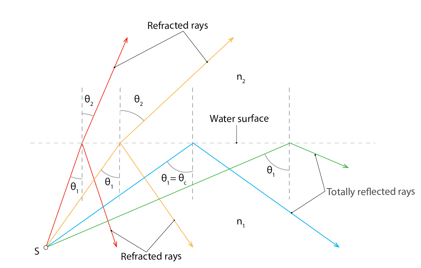 ) and the onset of total internal reflection (
 ) (adapted from Keller et al, 1992)
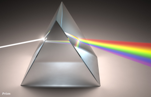
Since we know from the wave equation that  it follows that light at different wavelengths will travel through a medium of glass at different velocities. Snell’s law tells us that this will lead to differences in refraction. Thus an incident beam of polychromatic white light will disperse, with different spectra being differently refracted, and emerging from a prism as bands of (essentially monochromatic) colours of light (violet, indigo, blue, green, yellow, orange, red). This effect was first discovered by Newton in 1672.
There are many instances in which these optical properties of transmission, reflection, refraction and total internal reflection can be employed to control and enhance the distribution of daylight in buildings.
6.3 Daylight
The daylight performance of buildings has conventionally been evaluated using a concept called the Daylight Factor. This is a simplified geometric concept which assumes that the sky has the same brightness in all directions, that it is isotropic. But we know from Chapter 2 “Solar geometry and radiation exchange” that this is not the case, that skies are in reality anisotropic. In this section, we will explore the daylight factor concept and the methods to calculate it, because this simplified concept is very helpful in understanding the various contributing factors to interior daylighting. We will then go on to discuss more sophisticated methods of daylight evaluation and their corresponding metrics that have recently been introduced and found widespread application in practice.
6.3.1 Daylight factor
The daylight factor is conceptually straightforward. It is simply the ratio of the daylight received on a horizontal plane (within a building) Ei relative to that received on an unobstructed external horizontal reference plane Eo, multiplied by 100:  , %. There are three component parts to this daylight factor, the Sky Component SC, The Externally Reflected Component ERC, and the Internally Reflected Component IRC, so that
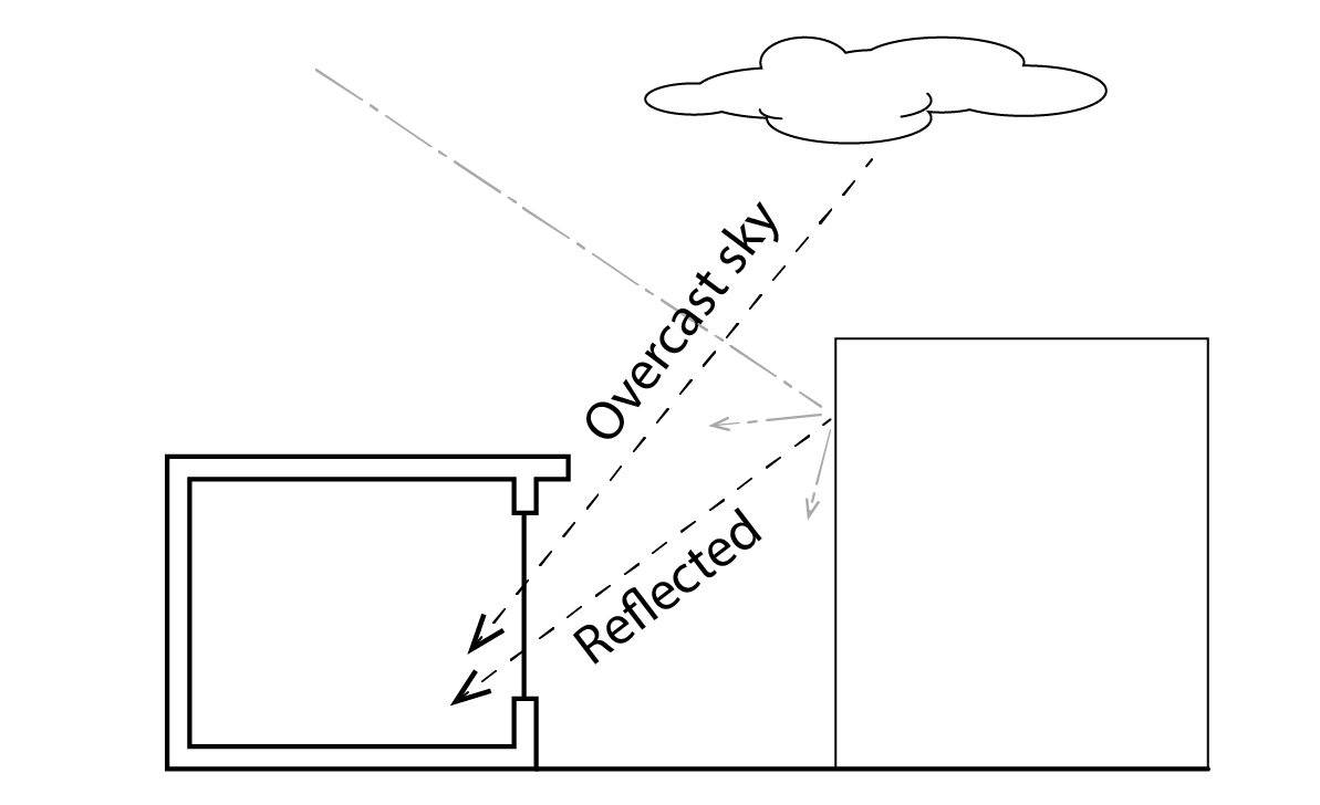
  . The external components are indicated in the following diagram. As one would expect, the sky component is received directly from the sky. The externally reflected component relates to the contribution of light that has been reflected from (normally building) surfaces that lie above the horizontal plane. It is often assumed that the brightness of these surfaces is around 10% of the brightness of the sky. Understandably therefore, there are daylight advantages to be gained by positioning buildings such that the sky component is maximised to the detriment of the externally reflected component. The internally reflected component relates to the luminous flux that is transmitted into our room, from both above and below the horizontal planes (so that the luminous flux from above enters in the downwards direction, and that from below enters in the upwards direction) and is then attenuated by reflection from the interior surfaces that comprise our room. Under normal circumstances, this internally reflected component IRC makes a relatively modest contribution to interior daylight levels.
The average daylight factor
The following simplified analytical expression has been formulated to calculate an average room daylight factor  , that is, the spatial average of the daylight factor throughout the working plane within a receiving room:
(5) 
in which  represents the average transmittance of the glass of area AG,
  represents the sky view angle, A is the total internal surface area and is the area-weighted average reflectance of the surfaces that comprise our room. The sky view angle is the angle subtended from the zenith to the mean angle of the adjacent urban horizon, call this
  , where
  , h is the mean height of this adjacent skyline above a point at the centre of our window and w is the width of the street from this point to the adjacent buildings that comprise this skyline. Ignoring any additional obstruction due to the reveal at the top of our window, our sky view angle is then:
  , and our mean reflectance
  .
.
Now, if we have in mind a target average daylight factor, we can re-arrange the above equation, to isolate the area of glazing that would be required to achieve this value:
(6) 
Measurement of daylight factor using an artificial sky
The daylight performance of rooms in buildings can be conveniently evaluated using a reduced-scale physical model. This is achieved by placing the model on a table within an artificial sky and measuring both the indoor illuminance and the outdoor illuminance using photocells (which convert the incident illuminance into an electrical output) connected to a lux metre, which itself converts the analogue voltage into an illuminance reading. There are two main types of artificial sky, mirrored skies and discretised sky vaults. The latter contain lamps that are supported by a frame that forms a hemisphere. Each of these lamps can be individually controlled by a computer to simulate overcast sky conditions as well as clear sky conditions and variations in between. Far more common are mirrored skies, which consist of a set of fluorescent tube lamps that light a small square shaped room from above via a diffusing fabric. The walls of this room, usually include a table to support the model at its centre, are comprised of polished mirrors. It is helpful to note at this point that even though there is little variation with azimuth, the brightness (or luminance, L) of overcast skies does vary with altitude, such that (Moon and Spencer, 1942):
(7) 
where  is a luminance at the sky zenith. We call this the standard overcast sky representation. Mirrored artificial skies emulate this standard sky, in which the zenith is three times brighter than the horizon.
The photocells are typically 16mm high, which corresponds to a working plan height of 800mm at a scale of 1:50. The floor of a model can be marked to represent a grid and one or more photocells placed within this grid, with a further photocell placed on the roof of the model. The lux metre can then indicate directly the daylight factor that is measured at each grid point.
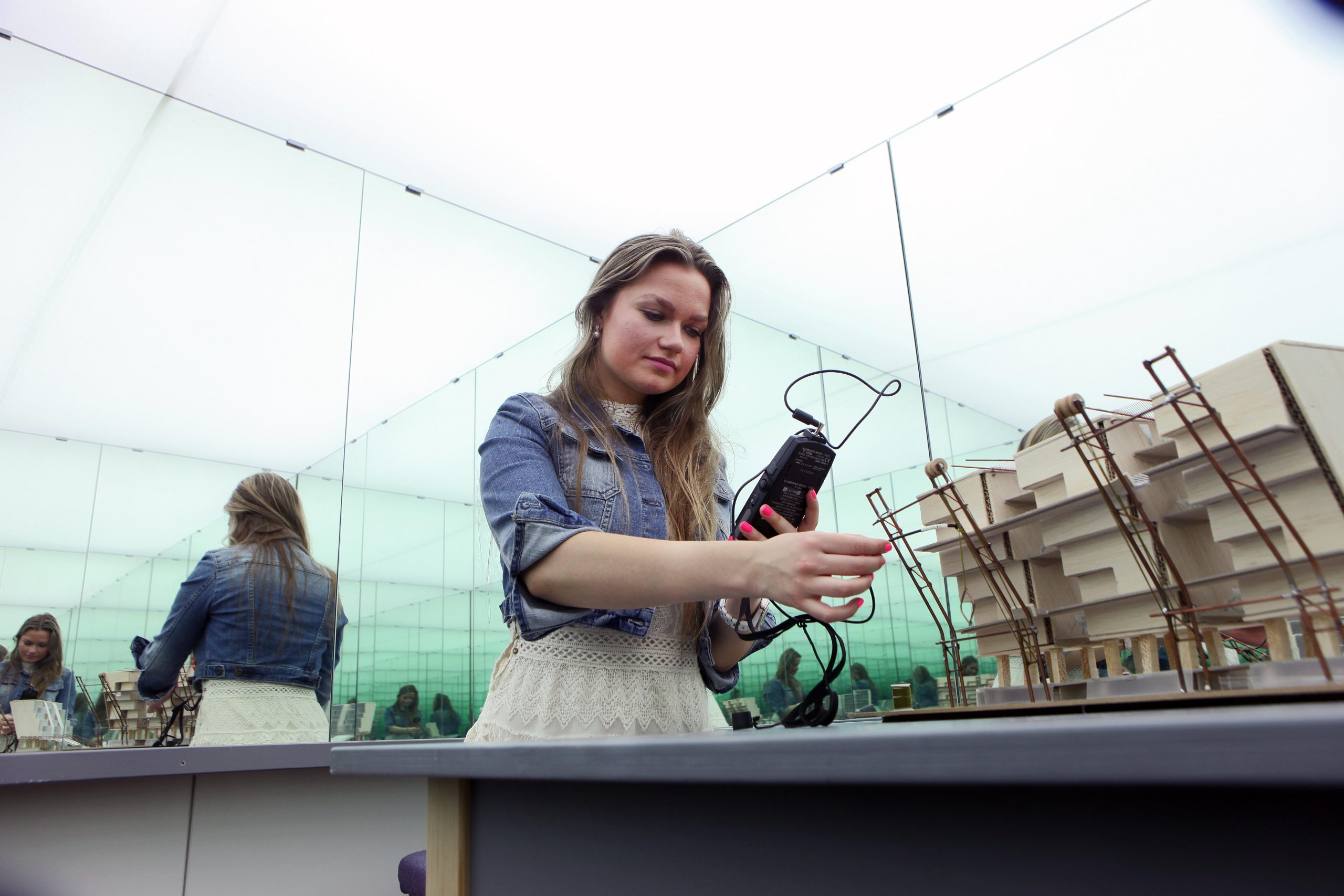
It is important to note that, when preparing a physical model for daylight evaluation purposes, the room needs to be fully sealed to prevent light leaks (though it is convenient to have a removable roof which overlaps the walls so that photocells can be easily repositioned), that the surfaces are finished using card with a reflectance (preferably also colour) that matches the intended finish and that glazing is represented using one or more layers of a flexible transparent material, such as acetate, to represent the transmission loss of the intended type of glazing. One advantage of physical modelling like this is that the interior can also be photographed, preferably using a fish-eye lens. It is however rather time consuming.
Calculation of daylight factor: a simplified case
Consider a window located at a distance D from a point on a horizontal working plane, located perpendicular to the centre of our window, which has a width W and a height H above this point. If we split this in half, our half-window has a width W/2. This geometry leads to the half-window subtending an altitude  , spanning an azimuth towards it’s lower extremity
  and an azimuth
  to its upper extremity.
Sky component
This half window subtends a solid angle  . But of course, we have a mirror image of this half window to the left of our calculation point, so that the entire window subtends a solid angle of:
(8) 
Dividing this by the solid angle subtended by a hemisphere ( Sr) we have a proportion which, when multiplied by 100, becomes a sky factor, SF (essentially the Sky Component, but for a uniformly overcast sky):
(9) 
We saw earlier, that the sky is three times brighter at the zenith than at the horizon. If we integrated this relationship over the hemisphere ( ), we can calculate an illuminance E from this unit zenith brightness sky (Hopkinson et al, 1966):
(10) 
However, for our purposes, we don’t need an absolute sky luminance. It is sufficient that we express our distribution as being relative to a zenith of unit brightness (). Thus, we can calculate a mean relative luminance for the region of sky that is visible through our window ( ):
):
(11) 
where  is the mean altitude of the region of the sky vault that is visible through our window.
Now that we have accounted for the luminance variation throughout the sky vault using the standard overcast sky definition, we can calculate our sky component for this simplified case:
(12) 
Where  represents the glass transmittance for our mean altitude
  , using the expression presented earlier for
  .
.
Externally reflected component
Suppose that we now have some obstructing buildings adjacent to our window, forming a continuous obstruction skyline, to a level h in our window, as viewed from our point D:
We can also calculate the solid angle for this obstructed region (indicated by shading above) using the same expressions as above, but substituting the expressions  and
and  , indicated by the two red arcs in the above diagram, thus:
  and
and  , so that now we can determine the solid angle of our externally reflected region as:
(13) 
we can also then calculate a corresponding externally reflected factor, EF:
(14) 
This we can also subtract from our prior expression for SF, leaving only that part that relates to the visible sky.
Now, our adjacent obstruction is at best going to have an unimpeded view of half of the sky vault (so that, at the mid-point of the reflecting wall that is visible from the point of interest in our receiving room it has a Sky Factor  of 0.5) and is likely to have a reflectance
  of around 0.2. Our mean obstruction luminance
  is then:
(15) 
So that we can now calculate the externally reflected component of the daylight factor, thus:
(16) 
Internally reflected component
The Building Research Establishment (then called the Building Research Station) developed (Hopkinson et al, 1966) a very neat approach that enables internally reflected light to be calculated in a relatively straightforward manner. In the first conceptual step, let us approximate the reflection characteristics of our room to that of a matt (so Lambertian surfaces) fully diffusing sphere. In this case, for an incoming luminous flux F (lm), incident on surfaces of reflectance , our internally reflected component takes the form of an infinite geometric series, for successive reflections of light:
(17) 
If we now split our room into two halves, a lower half (L) and an upper half (U), each having its own average reflectance (because floors typically have far lower reflectances than ceilings do, for example), and we similarly split our incoming luminous flux F into that entering our room in the downwards direction D and that entering in the upwards direction U then we have an equation of the form:
(18) 
This is referred to as the BRS Split Flux Equation, since it splits the incoming fluxes into that incoming in the upwards direction which is first reflected from the upper half of the room and that incoming in the downwards direction where it is first reflected from the lower half of the room. Subsequent reflections are handled using the diffusing sphere approximation.
This tends to be implemented in the following way:
(19) 
where AG is the area of glazing (m2)  is the total internal surface area (m2),
  is the area-weighted mean reflectance of these indoor surfaces, CD is a downwards configuration factor and CU is an upwards configuration factor. The reflectances fw and cw refer to the area-weighted average reflectances of the lower (floor and wall) and upper (ceiling and wall) halves of our room respectively – see the diagram below.
All that remains then, is to calculate our configuration factors (CD, CU), our basis for determining the incoming luminous flux.
In harmony with the approach to determining the luminance of external reflected sources of light, we can assume that our ground has a Sky Factor (SFg) of 0.5, since the facade that light is reflected onto obscures around half of the vault, and we can also assume that it has a relatively low reflectance ( ) of around 0.1, so that:
(20) 
Determination of the downwards configuration factor is more complex, as this requires that the incoming flux from both sky and external reflections is modelled. Although we have the information to do this, through the modelling of SC and ERC, the Building Research Establishment has published tables of CD as a function of adjacent urban obstruction angle (we referred to this as in the average daylight factor section). From these tables, the following third order polynomial has been derived:
(21) 
Finally, our daylight factor is simply the sum of the three component parts:
(22) 
This describes the daylight model that is used within the lighting and thermal (LT) method, which is a simplified energy model of non-domestic building energy use (Baker and Steemers, 1999). It also provides the conceptual basis of the relatively more sophisticated dynamic model (Robinson and Stone, 2006) that is used within the urban energy modelling platforms SUNtool (Robinson et al, 2006) and CitySim (Robinson et al, 2009, Robinson, 2011). This dynamic model, and its implementations, was developed to simulate hourly daylight levels and associated artificial lighting energy use (of which more later) in tens, hundreds or thousands of buildings simultaneously.
However, if the objective is to model the distribution of daylight, even dynamically, in a single building, then there are very sophisticated and now easy-to-use simulation tools that employ more meaningful daylight evaluation metrics.
Strengths and limitations of the Daylight Factor
The Daylight Factor approach to daylight performance evaluation was developed in the 1960s when performing computational tasks was complex, tedious and time-consuming. It was attractive then to develop an evaluation technique for which there was a direct analytical solution that was not too computationally burdensome. The daylight factor is essentially a geometric model for which there is such a direct analytical solution. This entails some simplifying assumptions. In particular, that:
- The sky is isotropic, or that its luminance varies only with altitude.
- The contribution from sunlight can be overlooked.
- All surfaces are perfectly diffusing Lambertian reflectors.
- Internal reflections can be effectively approximated as a perfectly diffusing sphere.
The latter two assumptions relate to the contribution of reflected light. Under normal circumstances  , so that the errors involved in these assumptions are relatively minor in nature (and in any case, most surfaces do predominantly diffusely reflect light). Except that is, when sunlight is involved (which relates to the second limitation). For example, there may be situations when an adjacent building facade that is oriented South is directly illuminated by the Sun, so that
  ; or indeed situations whereby the sun is at a low altitude (so that the cosine of the angle of incidence on a horizontal place is large) and is significantly illuminating internal walls, so that
  . However, these situations are relatively unusual. Protagonists of the daylight factor would also argue that in the presence of sunlight, indoor illuminances – even ignoring the contribution from sunlight – are likely to be significantly above a threshold at which artificial lighting is required so that, at least for the purposes of energy calculations (of which more later) this can be ignored. Indeed, it may be that blinds are deployed to prevent glare due to excess sunlight illumination. The protagonists then would argue persuasively that assumptions 2, 3 and 4 are reasonable. But what of the first assumption? Are skies consistently overcast and does it matter if they’re not?
Shown below is a chart that illustrates the distribution of sky clearness index for the cities of Athens, London and Helsinki, calculated using a model due to Perez et al (1990). This clearness index (x-axis) progresses from 1 (overcast) to 8 (clear), and the y-axis indicates the number of hours that each clearness index is encountered at each location. The distributions for London and Helsinki are relatively similar, but the sky conditions in Athens are significantly more skewed towards being clear; though in all cases, complete clearness is relatively unusual. The important point is that, even for London, the sky conditions are overcast for 37% of the year (the remaining 63% being non-overcast) and this reduces to just 16% for the relatively sunnier location of Athens. So sky conditions do seem to matter. They affect both the magnitude and the distribution of sky luminance with corresponding implications for indoor illumination, visual comfort and the control of artificial lighting, with associated energy use consequences.
The limitations of the Daylight Factor approach can be overcome using modern lighting simulation techniques, which offer the additional benefit of being able to produce both useful and beautiful renderings of indoor spaces.
6.3.2 Simulation-based techniques and climate-based metrics
Simulation-based daylight analysis techniques normally use one of two methods, radiosity or ray-tracing calculations; though occasionally, hybrids of these techniques are employed. These techniques form the basis of modern computer graphics and underpin gaming and computer generated images that are used in special effects in film making. They both require three-dimensional models of the objects to be simulated and descriptions of the characteristics of the surfaces of these objects, including both transparent and translucent media such as glass or water, as well as descriptions of the sources of direct and diffuse light. They are capable of producing qualitative images of a staggeringly high, even photorealistic, quality. Many of them can also produce quantitative information, support the production of false-coloured images of illuminance or luminance distribution and the quantification of these variables at discrete points in a scene being simulated. This section describes, in brief, both types of program, in addition to some recent metrics that have been developed to accompany them, to facilitate evaluation of the usefulness of a building’s daylight design, both spatially and temporally.
Radiosity programs
Radiosity programs discretise the surfaces that form the three dimensional model of the scene that is to be simulated into a surface mesh of patches. This is usually a regular Cartesian mesh, comprised of square or rectilinear patches. Each of these patches acts as both a receiver of radiant energy and as a source or emitter. Reflections between source and received patches are assumed to be perfectly diffuse, they are Lambertian surfaces.
For the purposes of explanation, let us first consider a hypothetical scene in which we have just two patches, i and j, and also a direct source of illumination that is visible to i but not to j. We have calculated the illuminance [lm/m2] incident on patch i and we know its reflectance , so that we can calculate its luminance,  [lm/(m2Sr)], as before. Given this initial luminance, we can now calculate the illuminance incident on our receiving patch Ej, as follows:

where  is the solid angle of patch j as viewed from patch i [Sr] and
  is the cosine of the angle of incidence from the centroid of patch i to the centroid of patch j. But now, patch j is the source for our receiver patch i, so that we must now solve for this luminous energy transfer after first having calculated a luminance for patch j in the same manner as before (
 ), as follows:

We repeat this process until there is a sufficiently small difference between the results for  , so that we need not continue further. This is the basis of radiosity simulations, but of course, these normally involve considerably more complex scenes, with many surfaces, discretised into many patches, and potentially involving many direct sources of illumination (note that in illumination [as distinct from thermal radiation applications] these are only sources, they do not participate as receivers).
In this more general case, the radiosity equation formulates our radiation / illumination exchange problem as:

where Ei is the initial radiosity of (or the amount of luminous (or radiant) energy leaving the ith patch) [W/m2], Bi is the final patch radiosity [W/m2],  is the patch reflectance and Fji is a form factor, the fraction of energy emitted from j that is received by i, BjAj is the total energy radiated by patch j of Area Aj [W]. Note that
  for all i (for a fully enclosed scene, as in an interior space), so that energy is conserved.
This then is an iterative process and needs to be conducted for each patch in turn. Solving this equation is achieved using linear algebra, expressing the component parts as matrices and vectors. However, for large and complex scenes these matrices can be very large with consequent implications for the computing resource that is required to solve them. On the plus side, however, the entire scene is solved simultaneously. This means that the result is independent from the view of the observer so that once a scene has been simulated, you can easily fly through the scene to inspect how it looks and performs.
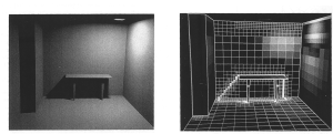
To enhance the quality of a rendered image, or indeed the accuracy of quantitative illumination calculations, radiosity algorithms tend to adaptively subdivide grid cells in locations where there are large gradients in their immediate neighbourhood (the neighbouring cells), for example, areas in shadow or at intersections between objects – see below.
Ray tracing programs
There are two types of ray tracing program, backwards and forwards. Backwards ray tracers simulate a scene from the viewpoint of a virtual observer, propagating rays into the scene, either sampling light sources or spawning other rays and so on in a recursive process. Forwards ray tracers take the opposite approach, simulating a scene from the sources of illumination, firing rays from these sources until the scene has been sufficiently resolved (see below). These are potentially very accurate, but also extremely resource intensive, as only a small fraction of the emitted rays reach the image plane. For daylighting purposes, backwards ray tracing using the Open Source program Radiance (Ward-Larsen, 1999) has come to dominate.
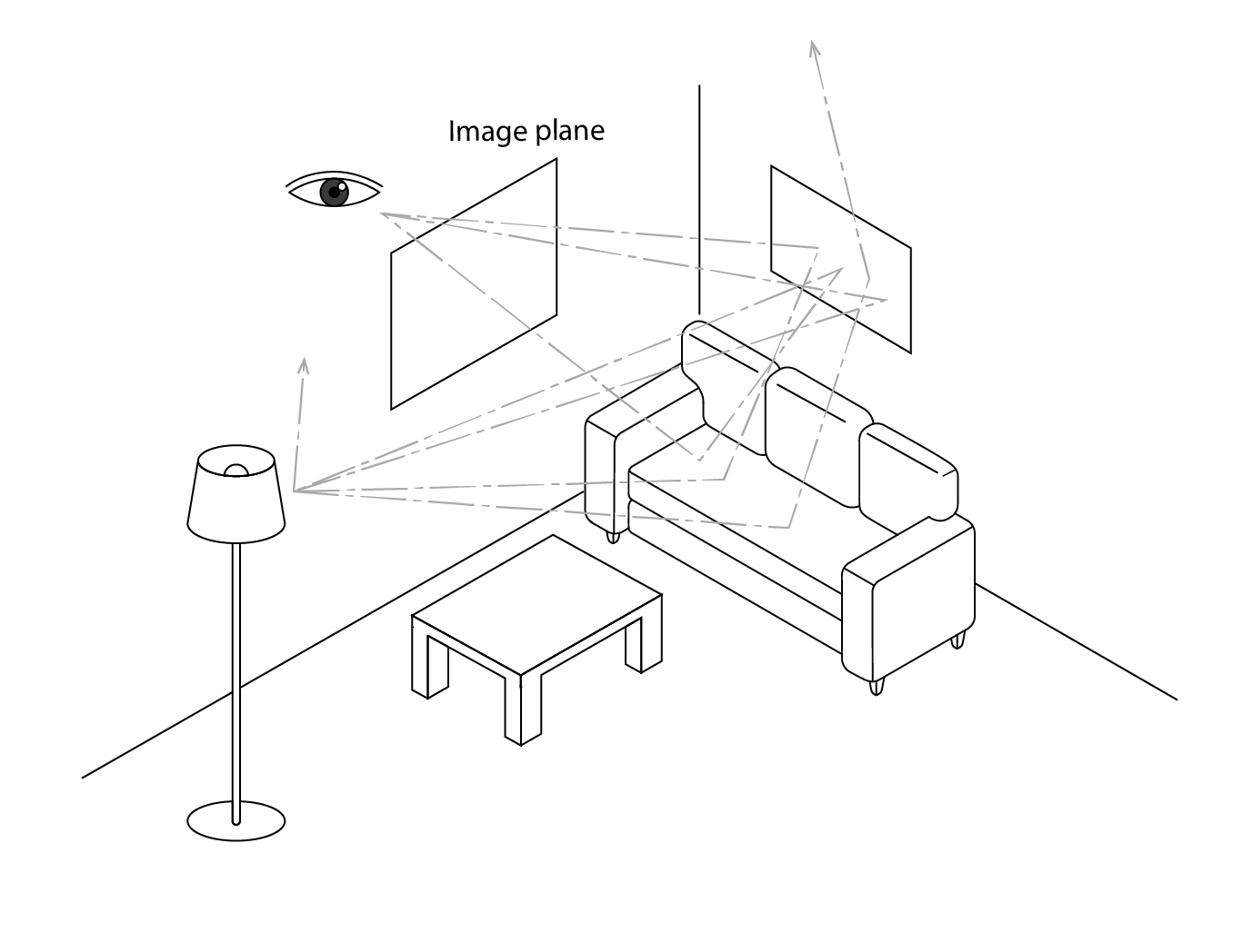
With a backwards ray tracer, somewhere within the three-dimensional scene to be simulated (or rendered), the modeller specifies the coordinates of a viewpoint. This is followed by a view direction and the dimensions of the image to be rendered. These three pieces of information are sufficient to define an image plane (as in the image below). From the viewpoint (represented by an eye below) eye rays (indicated by the path E in image below) are fired towards the image plane, passing through this (indicated by a kind of window below) and into the scene. This eye ray hits a transparent object. First, this leads to two shadow / light source rays being spawned, S1 successfully reaches light source LA, but S2 intersects with an obstruction (4) before reaching LB. A reflection ray R1 is also spawned from our transparent surface, which itself meets a transparent object, spawning its own transparency, shadow and reflection rays. Our eye ray also spawns a transparency ray, which passes through the transparent object and meets object 6. This in turn spawns two shadow rays, which meet both LA and LB. It also spawns a reflection ray R2, which will itself also spawn further rays.
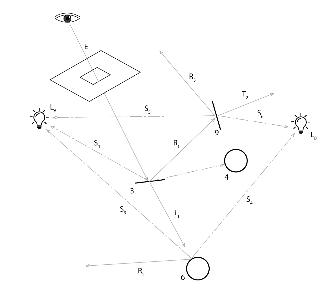
The path taken from an eye ray to a shadow ray that meets a light source (e.g. the sun, sky or an artificial light source) has a colour that depends on the characteristics of that source, and the transparency and reflectance characteristics of the objects that are intersected along this path. In this way, the following Radiance equation is solved:

where  is the reflected radiance,
  is the direct component arising from shadow rays from the image plane that successfully meets a light source, and the double integral describes the incident radiance and how this is modified by a bi-directional reflectance/transmittance distribution function
  . Since
  is defined in terms of itself (effecting
  ), this captures the recursive process which ceases when: the intersected surface is a light source, the ray has reflected more than a pre-defined number of times, the ray weight (the product of all previous reflectances) is below some threshold (e.g. ~0.005).
In line with radiosity algorithms, the ray tracing algorithm spawns more rays in regions of high contrast in illumination within the image plane (e.g. around the edges of a window in a room), so that the rendered image is better resolved.
The main benefit of radiosity programs is the drawback of ray tracing programs. The solution to illuminance / irradiance distribution is dependent upon the position of the observer and their view direction, so that fly-throughs are only possible by discretising the journey and performing multiple simulations, but this must be pre-configured. However, for this reason, they can be much quicker in their computations and they can handle both specular and diffuse reflections.
Climate-based daylight metrics
In contrast to daylight factor models that are bound to simplistic representations of overcast sky luminance distributions, simulation techniques open the prospect of modelling realistic sky brightness distributions which vary hour by hour. For example, the model due to Perez et al (1993) can calculate a sky luminance distribution based on measured solar radiation data (the standard data from a weather file) using a statistical model based on thousands of sky luminance distribution scans. This means that for every hour of the year, we can calculate an accurate indoor spatial illuminance distribution and thus determine the proportion of the working plane that meets a target level of illumination. This is the basis of climate-based daylight modelling (CBDM) and the metrics associated with this technique (Brembilla and Mardaljevic, 2019).
The two most commonly employed metrics are the useful daylight index (UDI) and the spatial Daylight Autonomy (sDA). The UDI is formed by a set of values, each representing the percentage of occupied hours where the illuminance level falls into certain ranges: 0–100 lux (UDI-n for not-sufficient), 100–300 lux (UDI-s for sufficient), 300–3000 lux (UDI-a for autonomous) and over 3000 lux (UDI-x for exceeded). The sum of these four categories must equal 100%. The sDA represents the portion of the working plane that complies with the Daylight Autonomy (DA) requirement; the percentage of occupied hours where the illuminance level is higher than a certain threshold (300 lux) for each spatial point. Both metrics are normally calculated throughout a grid so that the working plane is discretised into a series of points at the grid cell centroids.
6.4 Technologies to enhance daylight penetration
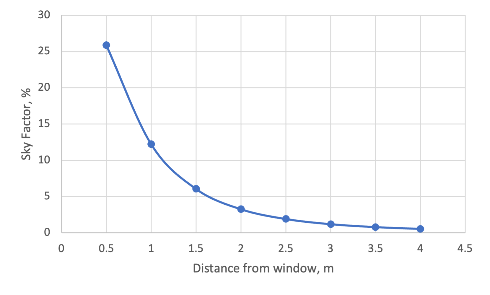
As the chart accompanying the solution to problem 5 below suggests, even in the absence of adjacent obstructions, the sky factor (and essentially therefore the Daylight Factor) decays exponentially with distance from a window wall. As such, the indoor illuminance may fall below a target threshold at a relatively small distance from this wall. In contrast, close to this window wall the working plane may have an excess of light or be subject to glare from the sun. To combat this over- and under- illumination a number of techniques and technologies have emerged.
The simplest of these is a light shelf (below), which simply reflects transmitted light, normally onto a ceiling from which it is diffusely reflected deeper into the room. This also reduces excess illumination near the window, so that a greater proportion of the working plane experiences useful daylight illuminance.
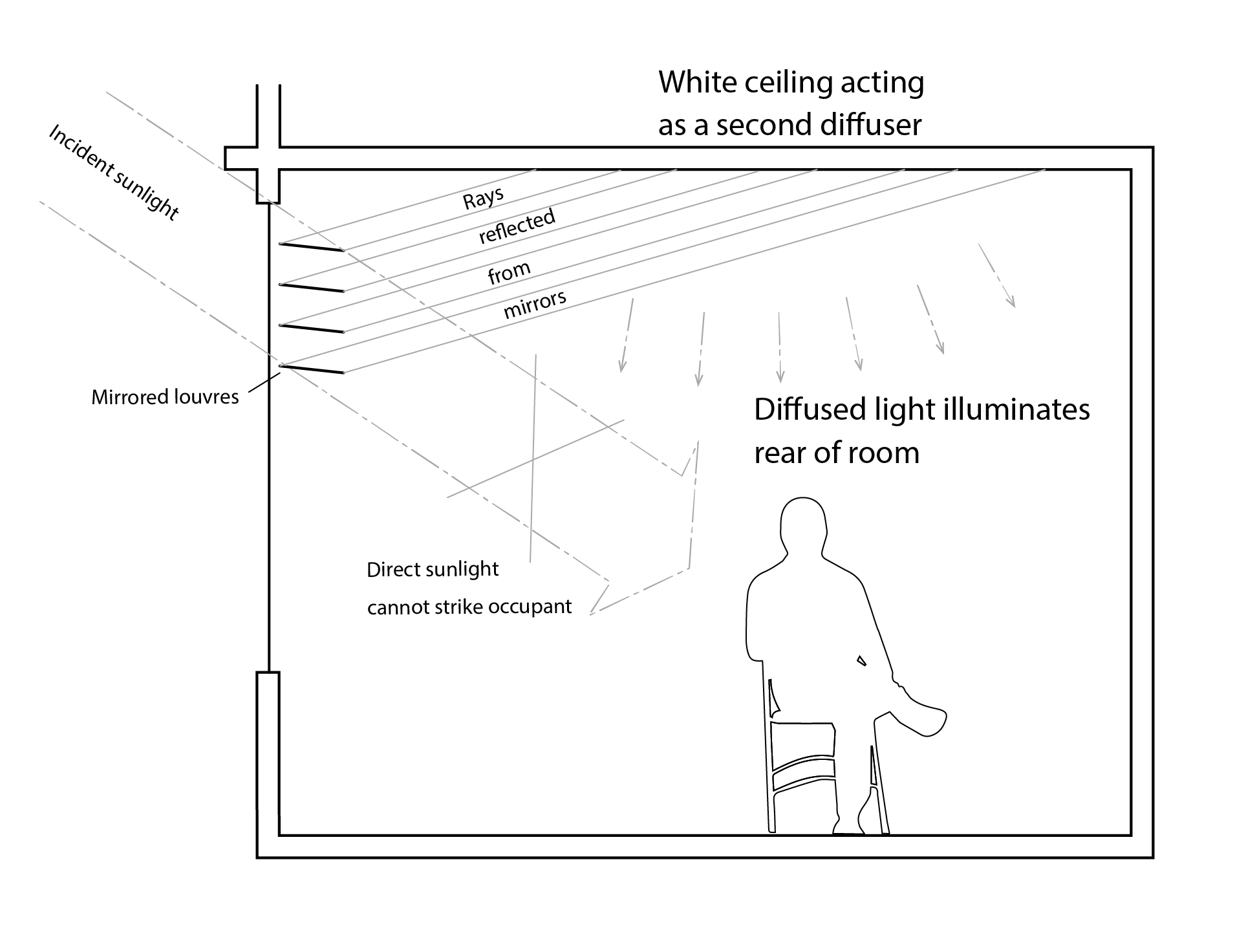
Internal light shelves are useful, but they do not enhance the amount of light (the total luminous flux) entering the space. For this, an external light shelf is required. Better yet, is an anidolic reflector (see below) which reflects diffuse light from throughout the sky vault as well as direct light from the sun both directly into the room as well indirectly following reflection from the ceiling. In this way, both the total transmitted luminous flux and the distribution of the transmitted light are enhanced.
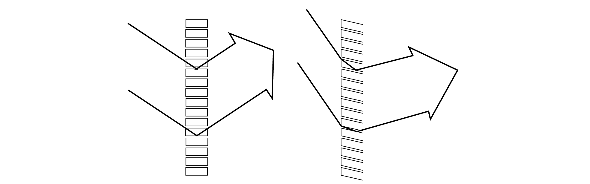
An alternative to using projecting reflectors is to use an alternative form of glazing. One option, shown below, is to use a transparent polymer material with grooves that are laser cut. This then creates interfaces between two media, polymer and air, enabling light to be totally internally reflected within the polymer, so that it exits at the inside face in an upwards direction. These grooves can be angled to bias particular directions of light, e.g. high altitude skylight or sunlight. This can be particularly effective in dense urban settings, with high skyline angles.
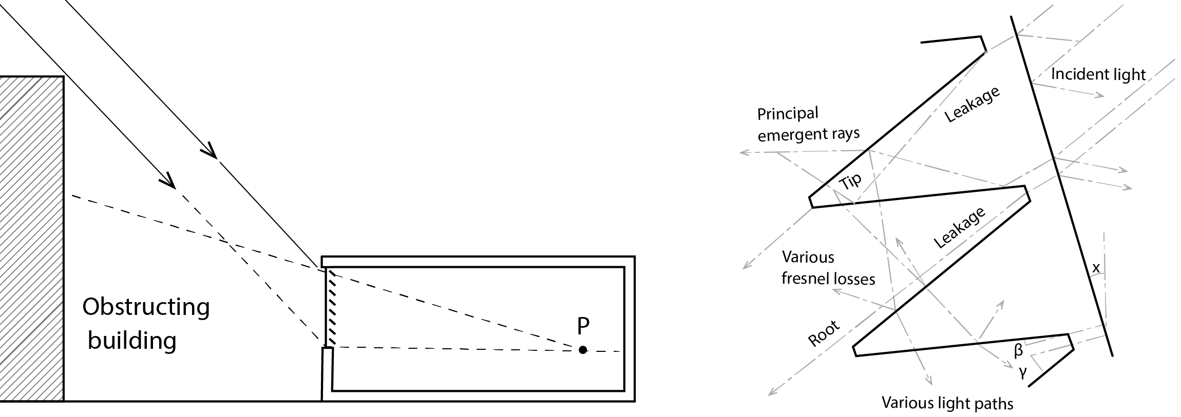
Prismatic glazing is another such option. In this case, there are more complex reflection and refraction pathways, determined by the sectional geometry of the glazing, but there is a dominant primary pathway (indicated as the principle emergent ray below) where transmitted rays emerge at a different and typically much shallower altitude than the angle of incidence on the outside face. Prismatic glazing can be very effective, but has the drawback that it hinders the view to the outside.
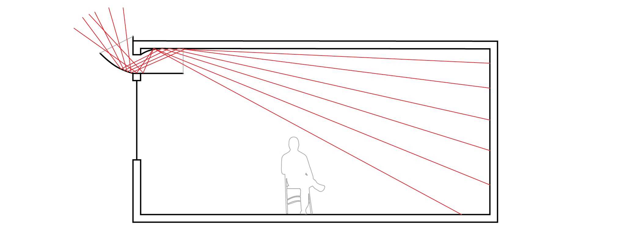
In relatively deep floor plates light pipes represent an attractive proposition, to harness light from the sky and/or sun, potentially using solar tracking mirrors and collimating lenses to ensure that the rays travelling through the light pipe are parallel to its walls to minimise reflective losses. Further mirrored reflectors can be used to channel light horizontally from the main vertical inlet – see below.
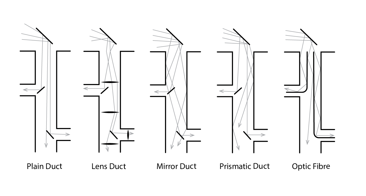
In a similar but more efficient vein, one can also use bundles of fibre optics (shown to the right in the above image), with sun-tracking concentrators directing bright light onto the outer face of these fibres. These can then be easily channelled in conduits through a building, without incurring losses due to bends in the fibres (due to total internal reflection within the fibre), to relatively distant unglazed spaces, where the outlet is directed towards a light-diffusing translucent material.
6.5 Integration with artificial lighting
As noted in the introduction to this chapter, it is important that measures of daylight and artificial lighting provision be integrated with one another, and that artificial light is controlled in such a way that it responds to available daylight. This typically requires a photocell fitted to the underside of a lamp that faces down towards the floor. This photocell then needs to be calibrated so that it switches off or dims the light output from the artificial lighting installation to maintain a target illuminance on the working plane. This can save a significant amount of energy.
Consider a room which has a target illuminance of 500 Lux and it has a mean daylight factor in the region of the room that is linked with photoresponsive light controls of 2%. Since we know that  , it follows that we could switch off our lights at an external illuminance of
  , in this case of 25kLux.
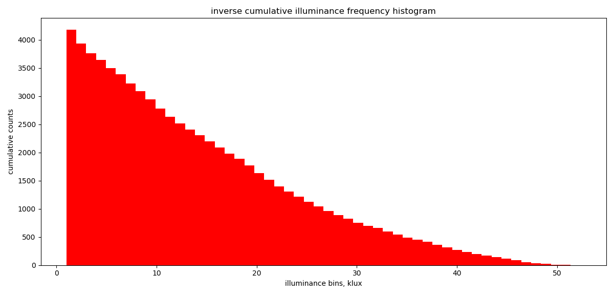
If we read along the x-axis in the image below and then up from 25kLux to where this intersects the top of our inverse cumulative distribution function (CDF) of illuminance and then across to our y-axes, we see that we could switch our lights off for around 1,100 hours. In other words for around a quarter of all daylight hours.
If we know what our installed lighting load is, in W/m2, then we can readily calculate the corresponding savings in artificial lighting energy use (Wh/m2).
6.6 Questions and worked examples
This section contains a series of worked examples or problems (P) and their solutions (S), as well as a series of written questions (Q) and their written answers (A).
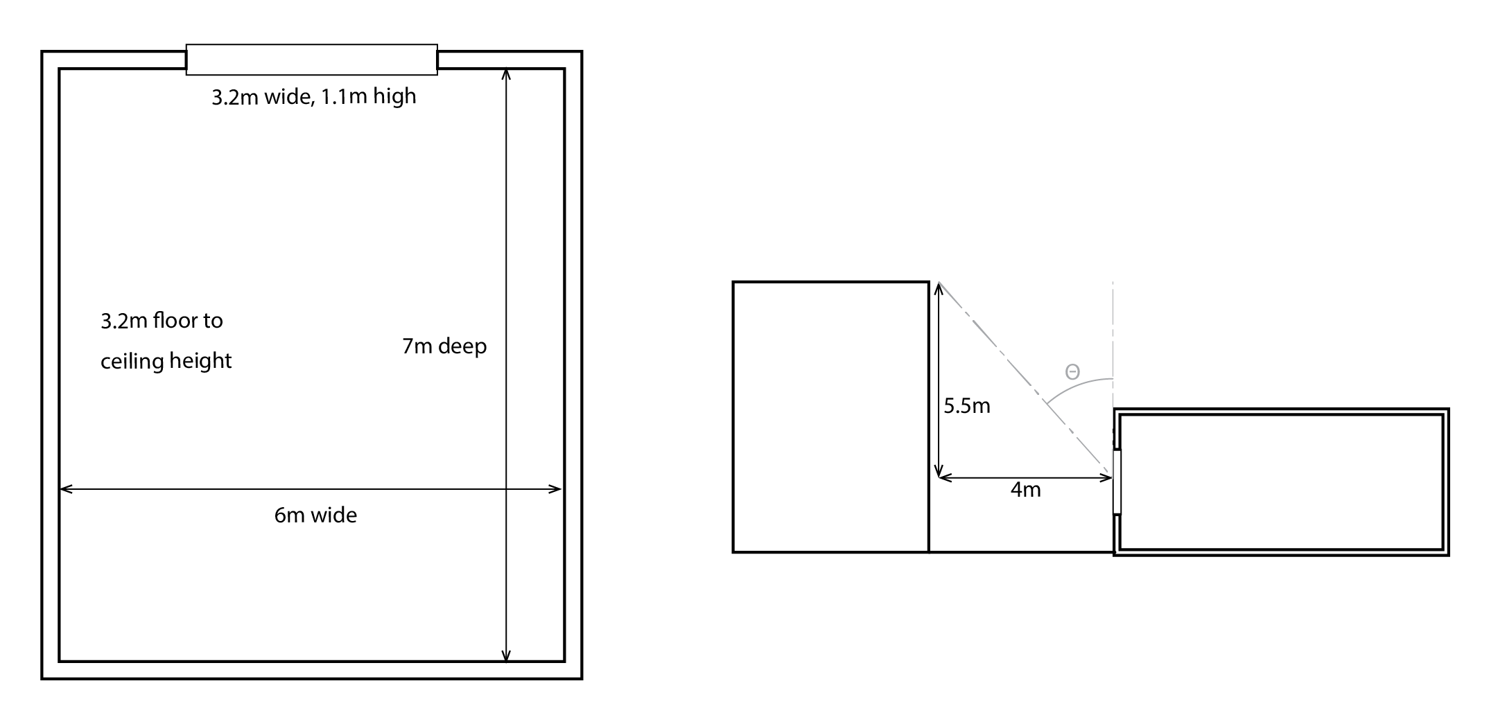
P1) The layout of a hypothetical office room (left) at the base of a street canyon (right) is illustrated below. The room’s reflectances are 0.7, 0.35 and 0.2 for the ceiling, walls and floor respectively and the glazing has a transmittance of 0.85. Calculate the average daylight factor and, assuming an external of 10kLux, calculate what the average indoor illuminance will be.
P2) For the scenario in P1, what happens if we increase the width of our window to 4m and we increase the reflectances of our Floor, Ceiling and Roof to 0.40, 0.75 and 0.55?
P3) For the scenario in P2, what if we were able to move our building back by 2m so that the distance between buildings is now 6m?
P3) Consider a large hypothetical window, that is viewed from a point p that is very close by; so close that you are essentially in line with the plane of the window. This window has a width of 10m, and a height of 10m, and you the observer at point p are just 0.001m from this window. Calculate the Sky Factor.
P4) Now repeat the calculation performed for P1, but for a more realistic situation of a window that is 2.5m wide, 1m high (above the working plane) and viewed from a point p that is 1.5m from the window plane. Calculate the Sky Factor for this case.
P5) Calculate a new Sky Factor for the above window geometry, viewed at a distance of 2.5m from the plane of the window.
S1) Our first task is to calculate our area-weighted mean room reflectance. Firstly, assuming that the glass reflectance  , we have a reflectance of 0.15. We can now calculate our areas and the mean reflectance:
| Surface | Surface area, m2 | Reflectance |
| Floor | 42.00 | 0.2 |
| Ceiling | 42.00 | 0.7 |
| Walls | 79.68 | 0.35 |
| Glass | 3.52 | 0.15 |
| Total | 167.2 | |
| Average | 0.40 |
We now need to calculate our sky visibility angle ( ), which is 36o. Inputting our parameters into the average daylight factor equation we have a value of 0.76% and a mean illuminance of 76Lux. This is likely to be inadequate!
S2) There is an improvement, but only by 0.4%, to a Daylight Factor 1.16% and a corresponding mean illuminance of 116 Lux.
S3) Our results are highly sensitive to this parameter, which considerably increases the sky visibility angle to 47o, so that our daylight factor increases to 1.53% and our mean illuminance to 153 Lux. This is likely to result in lights being switched off for a considerable period of time, particularly in the street-facing half of the room.
S4) To calculate our Sky Factor, we must first calculate the total solid angle of the two halves of our window from our point p:  . Taking each component in turn, we find that
  = 1.571 radians, = 0.464 radians and that = 1.571 radians. Using these results our total solid angle is 3.141 Sr and our sky component is 49.99%. We are so close to the window, that we can see very nearly half of the entire sky vault!
S5) For this new case, our values for  are respectively, 0.695, 0.606 and 0.588. Our solid angle is 0.381 and our Sky Factor is a more realistic 6.06%.
S6) By increasing our viewing point distance from 1.5m to 2.5m our Sky Factor has reduced to just 1.91%. This indicates that the daylight factor is highly sensitive to the distance from the window. In fact, if we repeat this process at 0.5m increments from the window, we have the following:
Q1) What is the colour of the skin of a Polar Bear?
A1) The skin of a Polar Bear is black, but it is covered in a dense network of translucent hair fibres. These are mostly hollow. When light is incident, some of this is internally reflected and transported to the dark absorbent skin and some of this is back-scattered, giving them a white appearance.
References
Baker, N. Steemers, K (1999), Energy and Environment in Architecture: A Technical Design Guide. Taylor and Francis.
Brembilla, E., Mardaljevic, J. (2019), Climate-Based Daylight Modelling for compliance verification: Benchmarking multiple state-of-the-art methods, Building and Environment 158 (2019) 151–164.
Hopkinson, R.G., Petherbridge, P., Longmore, J., (1966). Daylighting. Heineman, London.
Keller, F.J., Gettys, W.E., Skove, M.J. (1993), Physics, second (international) edition, McGraw-Hill.
Lechner, N., (1991), Heating, cooling, lighting – design methods for architects, Wiley.
Moon, P. and Spencer, D. E. (1942) ‘Illumination from a non-uniform sky’, Illuminating
Engineering, vol 37, no 10, pp707–726
Perez, R., Ineichen, P., Seals, R. (1990), Modelling daylight availability and irradiance components from direct and global irradiance, Solar Energy 44(5) p271- 289, 1990.
Perez, R., Seals, R. and Michalsky, J. (1993) ‘All-weather model for sky luminance distribution – preliminary configuration and validation’, Solar Energy, vol 50, no 3, pp235–243
Robinson, D., Stone, A. (2006), Internal illumination prediction based on a simplified radiosity algorithm, Solar Energy, 80(3) 260-267.
Robinson, D., Campbell, N., Gaiser, W., Kabel, K., Le-Mouele, A., Morel, N., Page, J., Stankovic, S., Stone, A. (2007), SUNtool – a new modelling paradigm for simulating and optimising urban sustainability, Solar Energy, 81(9), p1196-1211.
Robinson, D., Haldi, F., Kämpf, J., Leroux, P., Perez, D., Rasheed, A., Wilke, U., City-Sim: Comprehensive micro-simulation of resource flows for sustainable urban planning, Proc. Eleventh Int. IBPSA Conf: Building Simulation 2009, Glasgow, UK.
Robinson, D. (2011), Computer modelling for sustainable urban design: physical principles, methods and their applications. Taylor & Francis: London.
Ward-Larsen, G., Shakespeare, R (1998), Rendering with Radiance: Art and Science of Lighting Visualization, Morgan Kaufmann, 1988
Further reading
Cohen, M.F., Wallace, J.R. (1993 ), Radiosity and Realistic Image Synthesis, Morgan Kaufmann, 1993.
Glassner, A.S. (Ed) (1995), An introduction to ray tracing, Morgan Kaufmann, 1989 (9th printing, 2002).
