Architectural acoustics

Darren Robinson

8 Architectural acoustics

Longitudinal waves of sound are detected by ears in the form of pressure fluctuations. Compared to the standard atmospheric pressure, of 101.325 kPa, these acoustic pressure fluctuations are small, ranging from just 2×10^-5 Pa (the threshold of hearing) to 20 Pa (the threshold of pain). These sound waves can be pleasurable, for example in the form of speech or music, but they can also be unwanted. We refer to this unwanted sound as noise, and sources of noise can be internal to buildings, for example in the form of machinery, or external in the form say of vehicular or air traffic. The envelope of a building can be designed and controlled to regulate the transmission of noise from external sources, and internal structures in the form of walls and floors / ceilings can also be designed to reduce the transmission of noise within buildings. Surface finishes also have a role to play. Surfaces that incorporate soft materials, such as fabrics, are efficient at absorbing sound. This has an impact on sound levels, but also on the rate at which sound decays. In the case of spoken sound, this can influence the intelligibility of speech, which can be particularly important in classrooms and auditoria. The source of noise can also be to some extent contained. For example, by fixing items of machinery to damping materials, such as rubber mounts, to limit the transmission of generated noise through the fabric of a building.

In this Chapter, we examine the principles of sound and noise transmission, how sound affects speech intelligibility and the appreciation of pleasurable sounds like music, as well as how to calculate the transmission of noise and the decay of sound levels in buildings to support the design of buildings that effectively minimise noise levels to within reasonable limits.

8.1 Principles of waves, sound and noise

Consider a speaker that is connected to a music system. The music system transmits electrical signals through a positive cable to the speaker, which in turn is also connected via a negative cable back to the music system. Within the speaker, an electrical coil is located within a magnetic field. This coil is displaced by the magnetic field, the amount depending upon the intensity of the electrical signal. This in turn changes the position of a diaphragm, essentially a paper cone, which the coil is connected to. When the diaphragm is moved forward, this causes the adjacent molecules of the gases from which air is comprised to be compressed (indicated by the regions of closely packed molecules below), increasing the pressure in this region. Similarly, when the diaphragm is moved backwards a region of lower pressure rarefaction (indicated by regions of loosely packed molecules below) is created. This longitudinal wave is transmitted in the plane perpendicular to the diaphragm, travelling in this case (see the diagram below) from the speaker towards the ear. Although this wave energy is transmitted, the gas molecules are not, they simply fluctuate about their mean position.

Figure 1: Longitudinal (harmonic) sound wave

When the sound wave reaches the human ear, the air pressure fluctuations are converted to nerve impulses which are transmitted to and processed by the brain and interpreted as something heard. The pressure that the ear experiences is a combination of both air ( $P_{atm}$ ) and acoustic pressure ( $P_{ac}$ ). The standard atmospheric air pressure is 101,325 Pa, whereas (as noted earlier) acoustic pressure spans a range of just 2×10^-5 (the threshold of hearing) to 20 Pa (the threshold of pain). Acoustic pressure fluctuations are thus comparatively very small.

The metric that we use to quantify sound is the sound pressure level L, which has units of decibels [dB]. This sound pressure level can be calculated using a sound metre, which measures the acoustic pressure P, using the following equation:

(1) $\begin{equation*} \begin{flalign} L = 20\log_{10}\frac{P}{P_o} \end{flalign} \end{equation*}$

in which $P_o$ corresponds to the pressure at the threshold of hearing, 2 x 10^-5 Pa. This then converts sound pressures that span a factor of 1,000,000 (20/2×10^-5) into a range of 120dB, which much better corresponds to the ear’s ability to discriminate between sound levels. It is worth noting that a doubling of sound pressure ( $20\log_{10} (2)$ ) leads to an increment of just 6dB. Some indicative types of sound and their corresponding range in L are presented in Table 1 below. Most of the sounds experienced in the built environment span a range of 40-80 dB.

Examples of types of sound for different ranges in sound pressure level
Range of sound pressure level, dB	Type of sound
120-140	Aircraft taking off
100-120	Chainsaw
90-100	Power tools (saw, drill)
80-90	Busy restaurant kitchen
70-80	Busy city street
50-60	Normal conversation
40-45	Quiet office
30-40	Quiet bedroom
10	Someone quietly whispering

Table 1: Examples of sounds and indicated ranges of L

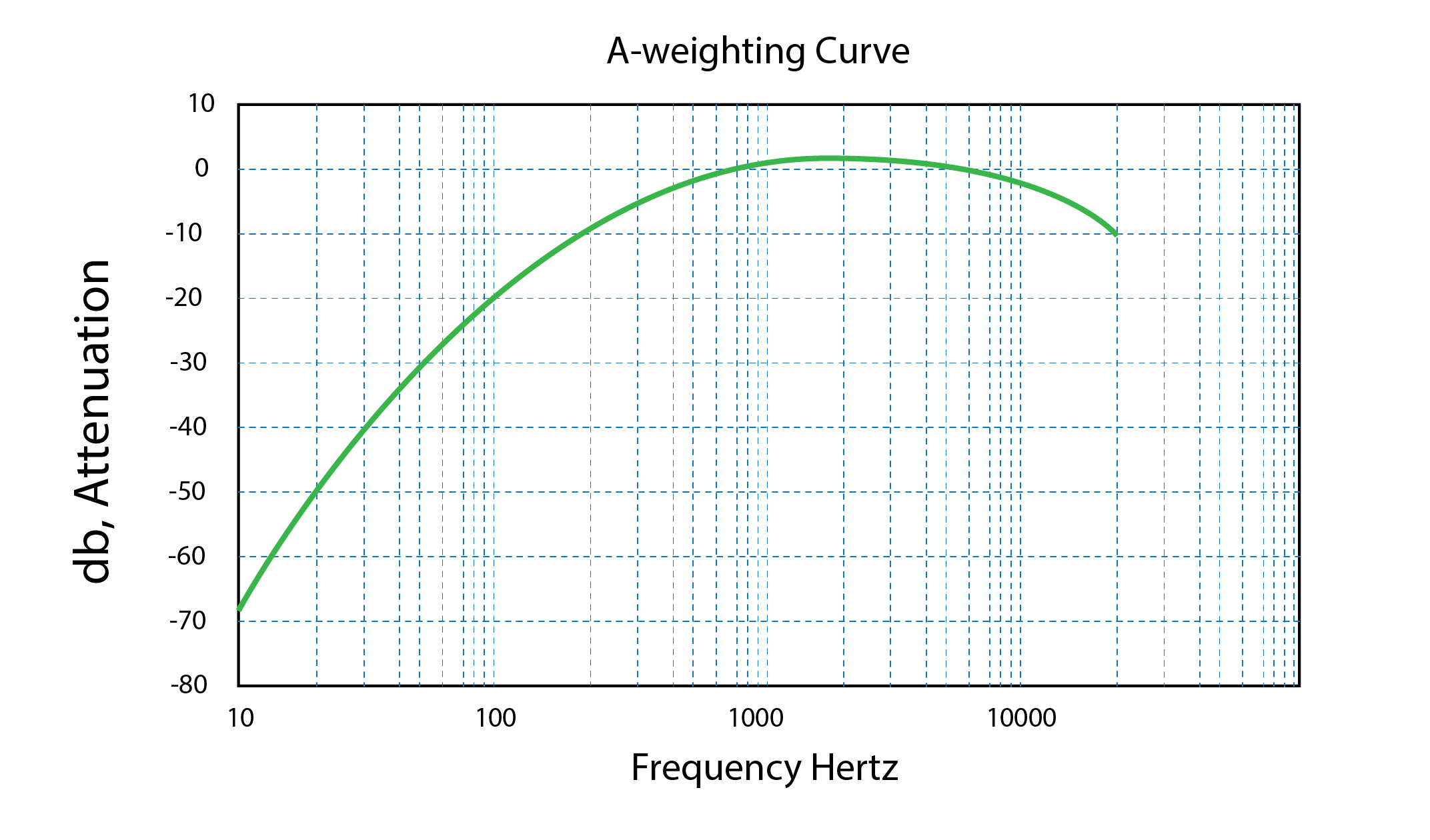
Sound level metres commonly use filters to adjust the transformation from acoustic pressure to sound pressure level. One such filter is the a-weighting, as presented below, which accounts for the human ear’s variation in sensitivity with frequency. We have a peak in sensitivity in the range of 1kHz to 4kHz, corresponding to the range of human speech and, at the higher frequencies, a baby’s crying. At higher and lower frequencies, the recorded sound pressure levels are attenuated by the filter, to account for reductions in perceived loudness. Sound pressure levels recorded using this filter are thus normally designated the unit of measure dBA, in which the A signifies the use of the A-weighted filter.

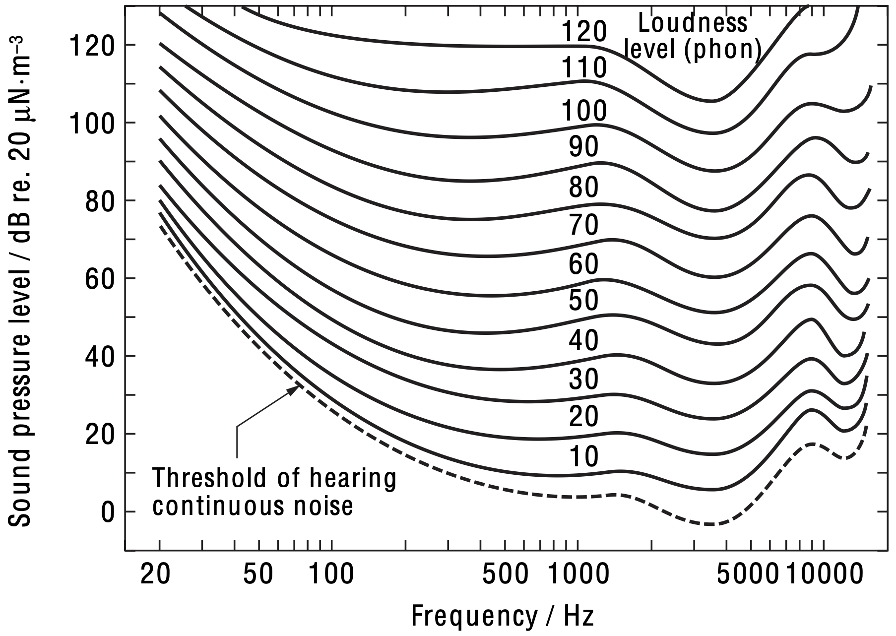
Figure 2: A-weighting curve, mimicking the human ear’s sensitivity

The following chart represents the sound pressure level that is required for an average listener to perceive a sound to be equal in loudness to that experienced at 1,000Hz. This leads to a considerable increase at lower frequencies.

Figure 3: Equal perceived loudness contours

Sound intensity I [W/m²] is also related to sound pressure P through the expression:

(2) $\begin{equation*} \left I=10\log_{10}\frac{P^2}{\rho C} \end{equation*}$

where $\rho$ is the density of air and C is the speed at which sound travels through air, typically 340 m/s. As with acoustic pressures, the sound pressure level can be calculated from the sound intensity:

(3) $\begin{equation*} \begin{flalign} L = 10\log_{10}\frac{I}{I_o} \end{flalign} \end{equation*}$

where the reference sound intensity ${I_o}$ is 10^-12W/m². A useful feature of this expression is that it enables us to calculate the sound pressure level resulting from the combination of distinct sound pressure levels, call this L_Tot, by adding their respective intensity ratios, where $\frac{I}{I_o} = 10^{L/10}$ , so that for a set of n distinct sound sources:

(4) $\begin{equation*} \begin{flalign} L_{Tot} = \sum \limits_{i=1}^n 10^{L_i/10} \end{flalign} \end{equation*}$

If we have a point source of sound, and that sound dissipates uniformly in all directions, then the sound intensity at a distance or radius r from the source location is: $I=\frac{P}{4\pi r^2}$ . If this distance is now doubled, so that $\frac{I_1}{I_2} = \frac{r_2^2}{r_1^2}$ , so that the reduction in sound pressure level $\Delta L$ is $10\log_{10}\frac{r_2^2}{r_1^2} = 20\log_{10}\frac{r_2}{r_1} = 20\log_{10}(2)$ = 6dB. Thus, any doubling of distance from a source of sound or noise (unwanted sound) leads to a reduction of sound pressure level of 6dB. In a similar manner, a doubling of sound intensity (say by combining two sounds of equal L) would lead to an increase in L of 3dB ( $\Delta L = 10\log_{10}\frac{2I}{I_o}$ ).

8.2 Reverberation and intelligibility

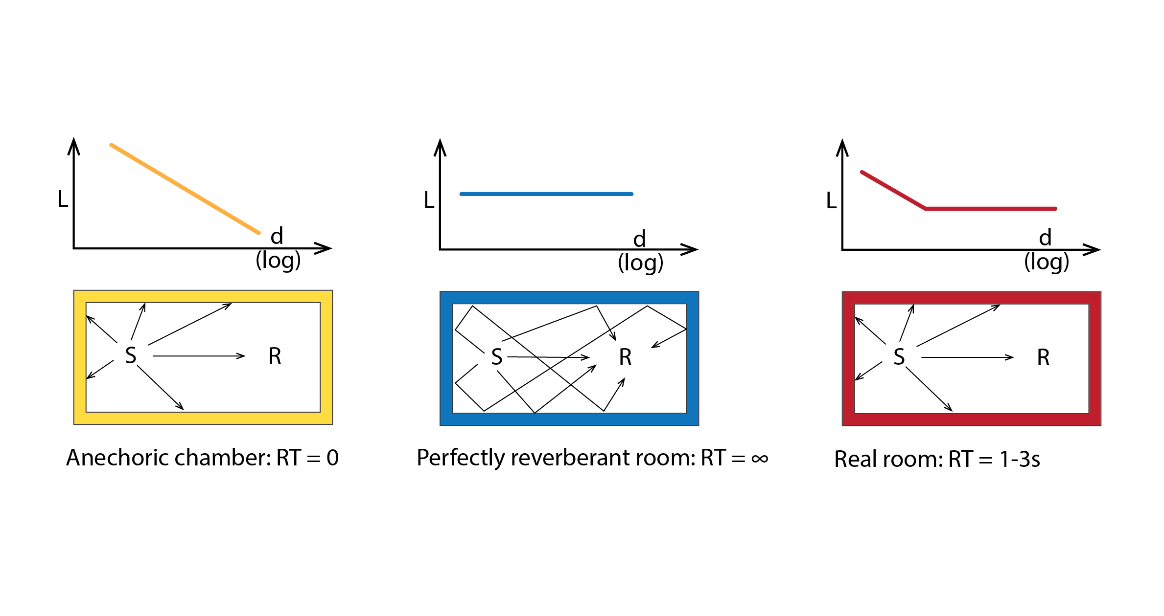
Shown below are three curves of sound pressure level L as a function of distance from a source of sound S. From left to right, these correspond to an anechoic chamber (which has perfectly absorbent interior surfaces), a perfectly reverberant room (which has perfectly reflecting surfaces) and a somewhat real room (which has partially absorbent / reflecting surfaces). In the first case, the sound level L recorded by a receiver R at a distance d meters from the source in proportion to $1/d^2$ , as the receiver only receives sound that is transmitted directly from the source – there is no reflected sound. In the second case, there is no reduction in sound level with distance from the source, as the sound is perfectly reflected from the room’s surfaces. If this source were a speech, that speech would be perceived by someone at location R as entirely incoherent, with all of the words’ consonants superimposed onto one another. The more realistic case exhibits a transition (exaggerated here) from a dominance of directly transmitted sound, to a dominance of reflected sound, as the receiver is progressively more distant from the source.

Figure 4: Hypothetical rooms of different reverberance

It is estimated that speech begins to become unintelligible when the delay in sound received from a reflected path relative to a direct path exceeds around 0.065s. With sound travelling at 340m/s in air, this corresponds to an increase in path length for the reflected case (e.g. from S to a point in a ceiling C from where sound is reflected to R) relative to the direct case (S to R), of 22m (SCR – SR = 22m).

Rooms can be characterised by how reflective or reverberant they are, by measuring or calculating their reverberation time. This is the time taken for sound intensity to decay to one-millionth of its initial value, or 60dB ( $\Delta L = 10 \log_{10}10^6 = 60dB$ ). When measured, this is normally based on what is referred to as the ‘interrupted sound method’. A source of sound that has a relatively equal intensity throughout the range of audible frequencies (we refer to this as pink noise, which closely resembles white noise) is emitted by a speaker and suddenly switched off. A sound level metre then records the time that the sound takes to decay, either by 60dB or (for the sake of a building’s occupants) by 30dB, this then being half of the full reverberation time, so that the calculated time must be doubled, for each octave band (normally 63, 125, 250, 500, 1,000, 2,000, 4,000, 8.000 Hz). Alternatively, this can be calculated using the following equation, which we refer to as Sabine’s equation:

(5) $\begin{equation*} \left RT=\frac{0.161V}{A} \end{equation*}$

where RT is the reverberation time (s), V is the room volume (m³) and A refers to the room’s total absorption, the product of the surface area S (m²) and the non-dimensional frequency-dependent absorption coefficient for the material from which this surface is comprised $\alpha$ (-); effectively, the efficiency with which the material absorbs sound. Thus, for a set of n surfaces (e.g. walls, floors, ceiling, windows, people (yes, we too absorb sound!), furnishings), the total absorption is:

(6) $\begin{equation*} \left A = \sum \limits_{i=1}^n S_i\cdot \alpha_i \end{equation*}$

Sabine’s equation assumes that the sound energy is evenly distributed over all of the surfaces of a room and that the sound is perfectly diffusely emitted (and reflected). Whilst this may not be precisely true in reality, the characteristics of most indoor spaces and the sounds emitted within them are generally sufficiently diffuse for this to be a reasonable approximation (rather like the Lambertian reflection assumption used in radiosity calculations^[1]).

Shown below are absorption coefficients for some common materials found within buildings.

Some examples of frequency-dependent surface absorption coefficient
Material	250 Hz	500 Hz	1000 Hz	2000 Hz	4000 Hz
Fair-faced concrete, plastered masonry	0.01	0.01	0.02	0.02	0.03
Fair-faced brisk	0.02	0.03	0.04	0.05	0.07
Painted concrete block	0.05	0.06	0.07	0.09	0.08
Windows, glass facades	0.08	0.05	0.04	0.03	0.02
Doors (timber)	0.10	0.08	0.08	0.08	0.08
Glazed tile / marble	0.01	0.01	0.01	0.02	0.02
Hard floor coverings (lino, parquet) on concrete	0.03	0.04	0.05	0.05	0.06
Soft floor coverings (carpet) on concrete	0.03	0.06	0.15	0.30	0.40

Most of the materials in the above table are relatively reflective (having low absorption coefficients), this changing little with frequency. An obvious exception, however, is the soft floor covering. This is an example of a porous absorbent material. Acoustic pressure fluctuations at the surface cause air to flow into and out of the pores of the material, with the resulting friction between the air molecules and the pore surfaces causing the dissipation of acoustic energy in the form of heat. Occasionally, membrane absorbers are employed. In this case, the acoustic pressure fluctuations provoke vibrations in the membrane, with the friction between the molecules of the membrane also causing acoustic energy to dissipate as heat. As shown in the table above, the acoustic pressure fluctuations at higher frequencies entail more dissipation of acoustic energy as heat, thus increasing the absorption coefficient.

The ideal reverberation time is around 1.5s for the purposes of speech intelligibility, though $0.5 \le RT \le 2.5$ is fine. Progressively higher reverberation times can lead to considerable reductions in speech intelligibility, as words and consonants become entangled, making it more difficult to discriminate between them. Conversely, this can be desirable in the case of music, causing the space to feel more ‘lively’.

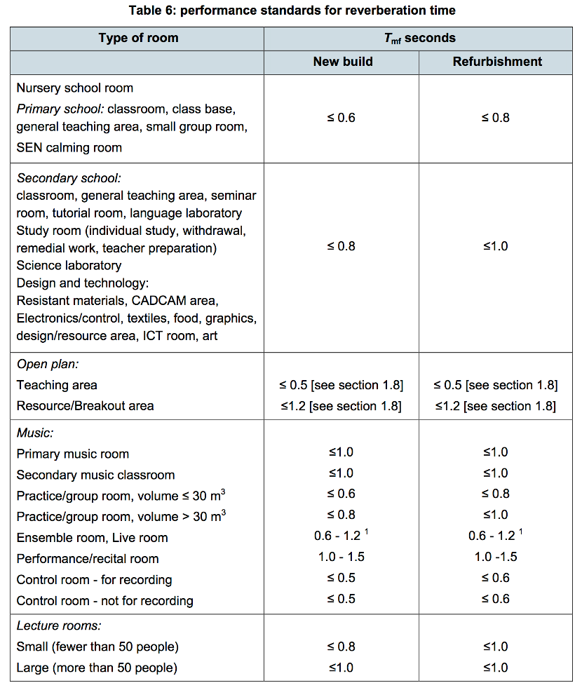
As an example, the following table (taken from BB93) provides examples of reverberation times that different types of space in a School building are expected to meet.

Figure 5: Standard reverberation times for different types of receiving room in Schools

8.3 Sound transmission and insulation

As noted in the introduction, noise is simply the presence of sounds that are unwanted by the listener. These noises may be airborne, for example in the case of speech, music or traffic, or structure-borne, for example arising from impacts with a structure (e.g. walking in shoes with heels on a hard floor covering) or vibrating machinery (e.g. a washing machine). The source of airborne noise may be internal or external.

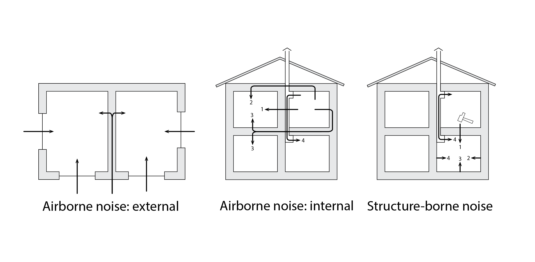
Figure 6: Types and modes of noise transmission

The above diagrams identify transmission pathways for the different types or sources of noise. External airborne noise (shown left, above) may be transmitted through windows (1), directly through walls (2), or indirectly through what we call flanking pathways (3); that is, via other structures (walls, floors) that are directly coupled to the external wall. Similarly, Indoor airborne noise may be transmitted directly via a separating wall (1), or indirectly via flanking pathways involving a ceiling (2) or a floor (3), or via a chimney or some other form of ductwork, such as a mechanical ventilation air duct. An impact provoking structure-borne noise may also be directly transmitted, for example via a floor (1), along a single flanking pathway to a coupled wall (2) or a double flanking pathway via the wall to a coupled floor (3), as well as via an attached duct (4).

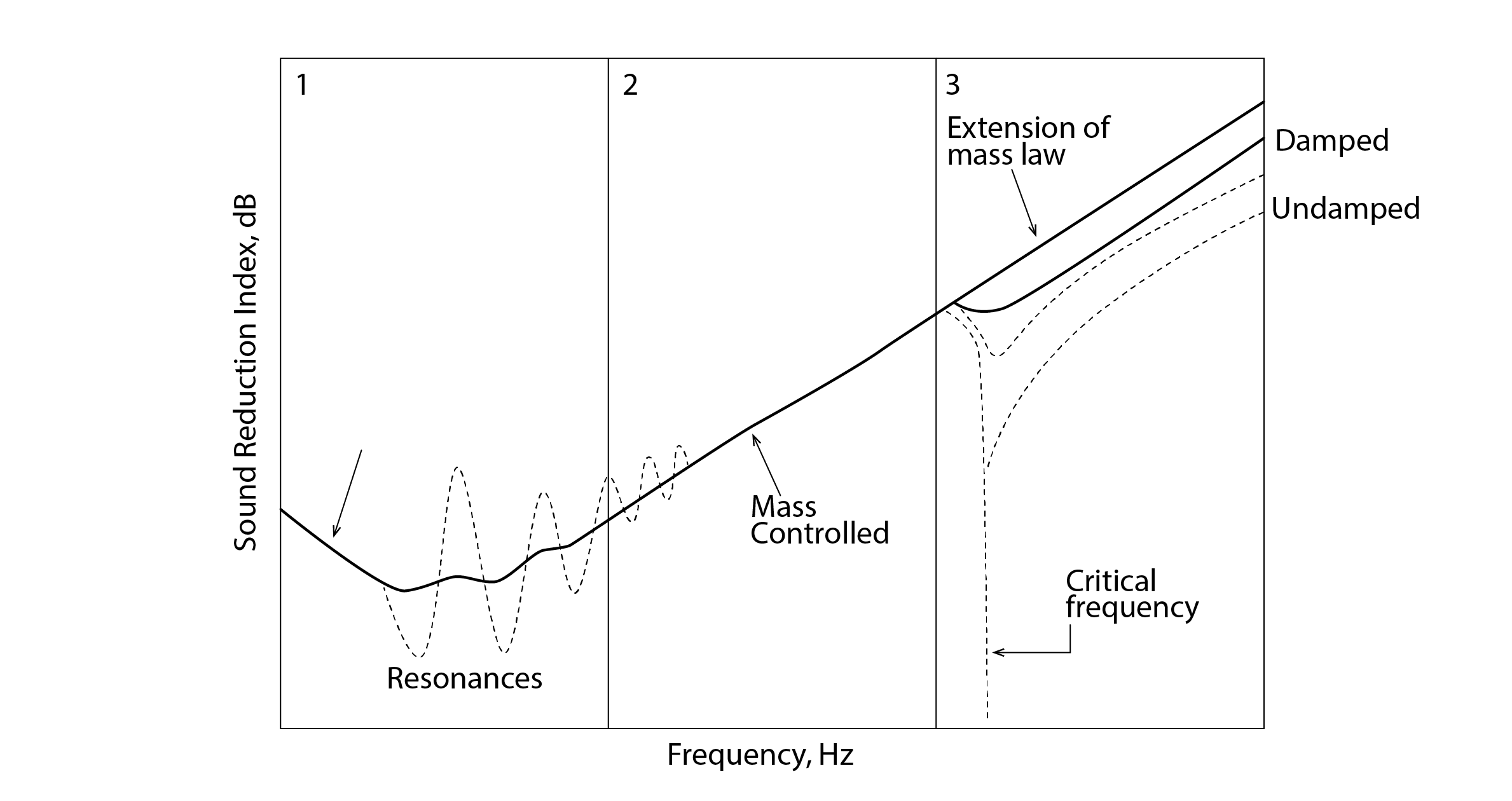
Whether a wall, a ceiling or a floor, the frequency-dependent behaviour of a single leaf partition is illustrated in the diagram below, where the y-axis represents the transmission loss of the partition (alternatively known as the partition’s Sound Reduction Index, or SRI, in dB). In the first region (1), which corresponds to lower incident sound frequencies, the partition’s behaviour is controlled by its stiffness, with the partition offering more resistance to vibration at lower frequencies. Within this region, localised increases and reductions to sound insulation may occur in situations where the frequency of the incident sound wave coincides with the natural frequency (or multiples thereof) at which the partition vibrates^[2]. Region 2 of this diagram is known as the mass-controlled region. At higher frequencies, the molecules from which the partition is comprised need to vibrate faster, causing the dissipation of acoustic energy in the form of heat, so that the partition is more effective at damping (or resisting) the transmission of sound. This increase in transmission loss, call this $\tau$ , is described by the following mass law of sound insulation:

(7) $\begin{equation*} \left \tau = 20 \log_{10}mf-k \end{equation*}$

where m is the surface density [kg/m²], f is the frequency (Hz) and k is a constant, usually taken to be 43dB. Thus, for each doubling of the panel’s mass or frequency of the incident sound waves, the transmission loss increases by $20\log_{10}(2) = 6$ dB.

The third region in this diagram is an extension of the mass law, except where there is a so-called coincidence dip. This occurs when the projected wavelength of the incident sound wave, $\lambda$ (recall that $\lambda = v/f$ ), is equal to the length of the flexural wave that is provoked within the structure of the panel itself. If the wave is incident at say $\theta^o$ from the panel’s surface normal, this dip occurs when the length of the wave provoked in the panel is $\lambda/\sin\theta$ .

Figure 7: Frequency-dependent behaviour of a typical single-leaf partition

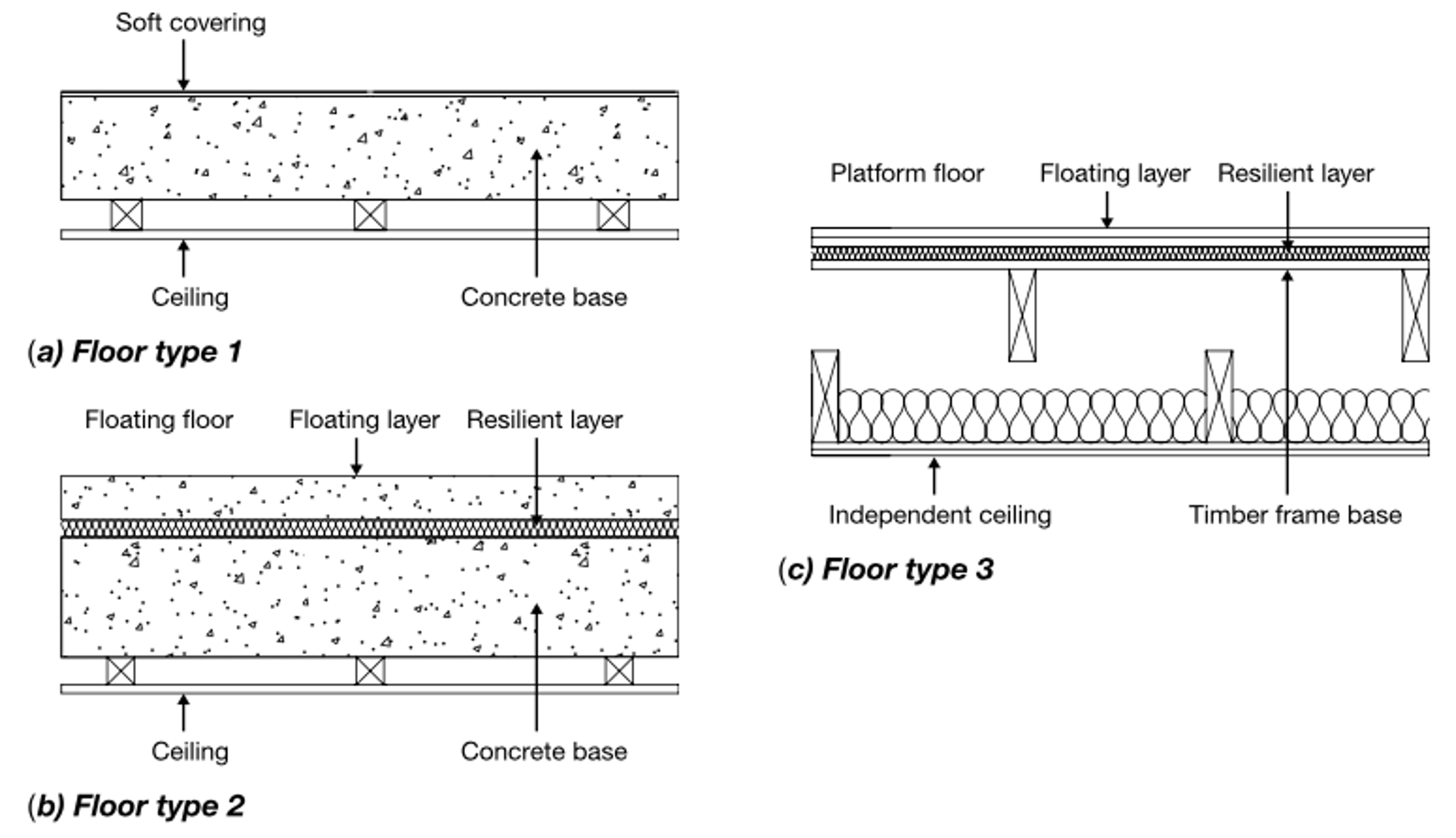
Now, floors in buildings may transmit both airborne and structure-borne noise. The following diagrams are taken from the Building Regulations Approved Document E as examples of constructions that are designed to impede the transmission of sound. In the case of floor type 1, the resistance to airborne sound depends mainly on the surface mass of the concrete base and, to a lesser extent, on the surface mass of the ceiling panel. The soft floor covering reduces the magnitude of impact sound at its source.

Floor type 2 below incorporates a floating layer (e.g. a cement-sand screed) which sits on top of a resilient layer of damping material. This could be a thick rubber or a layer of expanded polystyrene. This is likely to be more effective still at the reduction of impact sounds than in the Type 1 case. Finally, in the case of timber framed structures, we have an acoustically separated combination of a floor and ceiling, supported by independent frames; the floor incorporates a floating surface layer and the cavity between floor and ceiling incorporates insulation to absorb airborne sounds that are transmitted from the floor to the ceiling (which may be exacerbated if standing waves are established in this cavity – of which more later).

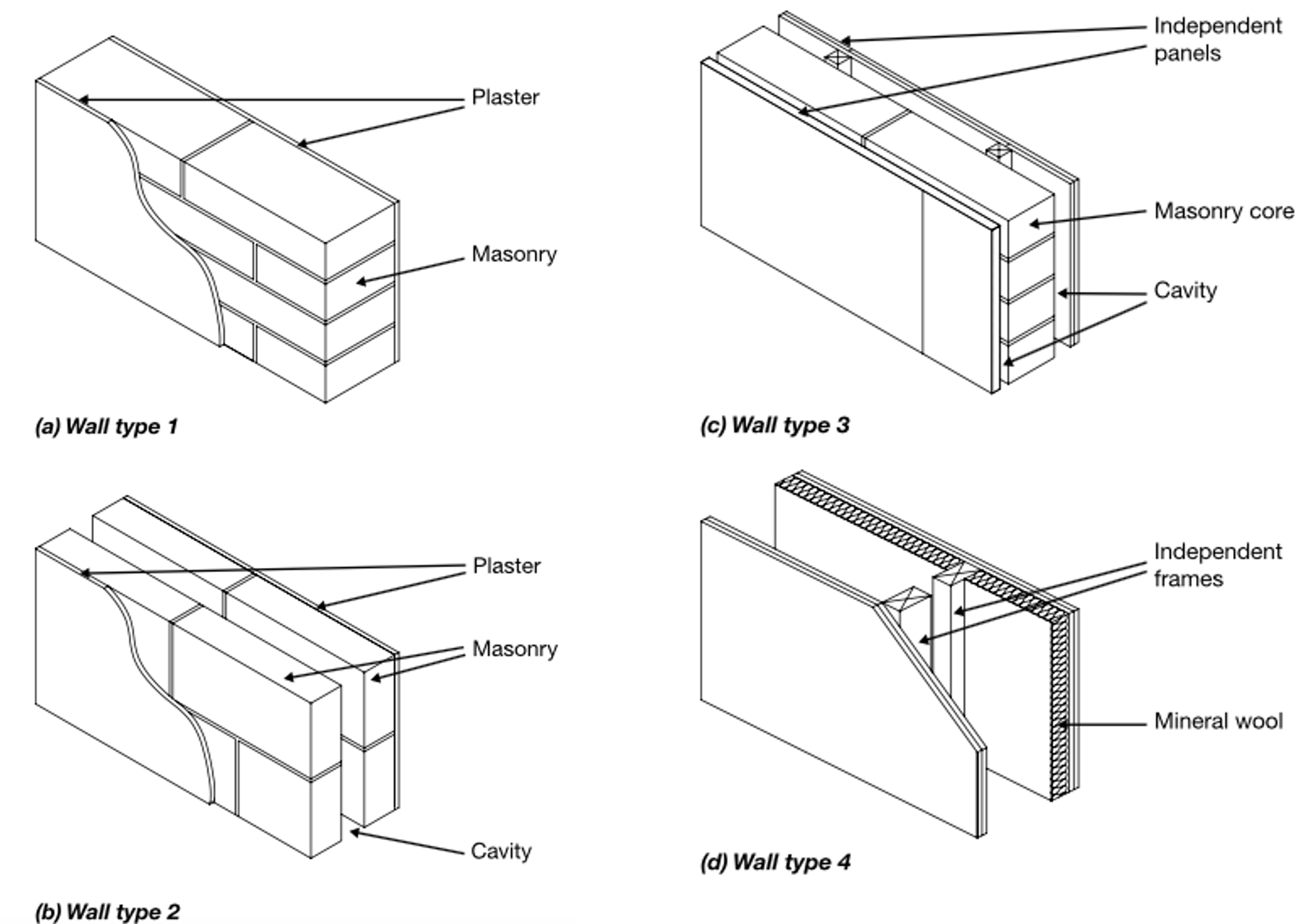
Figure 8: Types of floor, designed to resist noise transmission

Also from the Building Regulations (HMSO, 2015), are the following recommended configurations of wall, where the focus is upon protection from airborne noise transmission. In the case of Wall type 1, resistance to noise transmission arises primarily from the surface density of the masonry wall, and to a lesser extent also from the two layers of plaster. In the case of Wall type 2, this resistance arises from the two leaves, which are also affected by the extent to which they are isolated from one another. Structural ties between the layers have the potential to compromise their effectiveness. The presence of insulation within the cavity can help to absorb the airborne transmission of noise from one face to another. Resistance to noise transmission from Wall type 3 is offered primarily by the masonry core, though this is supplemented by the additional panels, which need to be supported independently from the core. Wall type 4 is similar in this regard, with two structurally independent layers and a porous absorber attached to one face within the cavity to absorb airborne noise propagation within the cavity.

Figure 9: Types of wall, designed to resist noise transmission

As noted earlier, in the case of single-layered panels, the acoustic integrity of the panel can be compromised when the frequency of the incident sound coincides with the natural frequency at which the panel resonates. In a similar manner, the integrity of a double-layered panel, such as a double-glazed window, can be compromised when standing waves are established within the cavity that coincide with its combined natural resonant frequency (or multiples thereof).

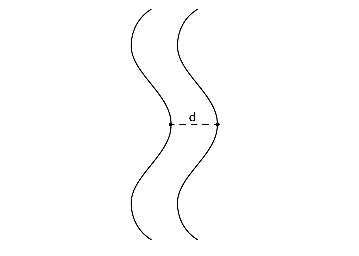
This resonant frequency $f_r$ can be calculated as follows:

(8) $\begin{equation*} \left f_r = k \sqrt{\frac{1}{d} (\frac{1}{m_1} + \frac{1}{m_2}) } \end{equation*}$

where d is the distance between the two leaves of the panel – the cavity width – (m), m is the surface mass of each of the two leaves (kg/m²) and k is a constant, having a value of 84. So, the larger the cavity or the greater the two masses, the lower will be the resonant frequency. This is helpful, as the ear is less sensitive at lower frequencies. Furthermore, the greater the difference in the two masses, the more effective is their combined damping. Thus, for good sound insulation, it is useful to specify large but differently massive layers, widely separated. As the table below demonstrates, acoustic windows follow this principle. Even the 8+4 combination offers considerably more resistance to noise transmission than the equivalent tripled–glazed case (4+4+4) which has an identical combined mass.

Acoustic properties of some multi-layered glazing assemblies
Glazing thickness, mm	Distance between layers, mm	Combined specific mass, kg/m²	Transmission loss, dB
Standard glazing
3+3	12	15	29
4+4	12	20	30
4+4+4	9	30	31
Acoustic glazing
8+4	18	30	36
10+4	18	35	38
10+6	20	40	41
12+10	20	55	48

In a cavity between two surfaces, such as two panes of glass, a resonant standing wave will be established where the sound within the cavity has a wavelength of twice its thickness, so that $\lambda = 2d$ . In the general case, standing waves may be established for multiples of half-wavelengths, n, so that $\lambda_n = \frac{2d}{n}$ . This may alternatively be expressed as a frequency, so that $f_n = \frac{v}{\lambda_n} = \frac {v \cdot n}{2d}$ . The presence of these standing waves considerably compromises the acoustic integrity of the assembly concerned (be this a cavity in a wall or a window); but the larger the cavity the lower the frequency and the lower the ear’s sensitivity to the corresponding reduction in transmission loss or sound insulation.

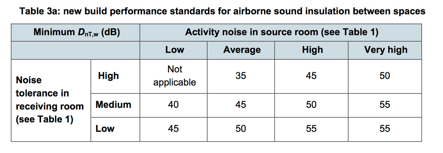
Within buildings, the amount of sound insulation that is required of partitions between rooms depends both on the amount of noise that is generated (the activity noise) within a source room, and on the degree of tolerance to noise in a receiving room. The table below presents the degree of sound insulation that is required of wall partitions between different types of space found in School buildings (taken from Building Bulletin 93 (Department for Education, 2015)). By way of example, a music practice room is likely to entail a very high degree of activity noise in the source room (the far right column) and an adjacent music recording studio is likely to entail a very low tolerance to noise (the bottom row). In this case, then, the amount of sound insulation that is required (the D_nT,w value) of a partition is 55dB.

Figure 11: Standards for airborne sound insulation between schoolrooms

This metric, the D_nT,w needs some explanation. The D refers to the difference in sound pressure level between the source room (L_s) and the receiving room (L_r), so that $D=L_s - L_r$ . The n in this metric refers to a normalisation with respect to the frequency-dependent reverberation time T in the receiving room, compared with a reference value:

Reference reverberation times as a function of room volume
*Reference reverberation time, T_o* (s)**	Room Volume, V (m³)
0.5	$V \le 100$
$\sqrt{V/400}$	$100 > V < 2,500$
2.5	$V \ge 2,500$

This leads to the following expression:

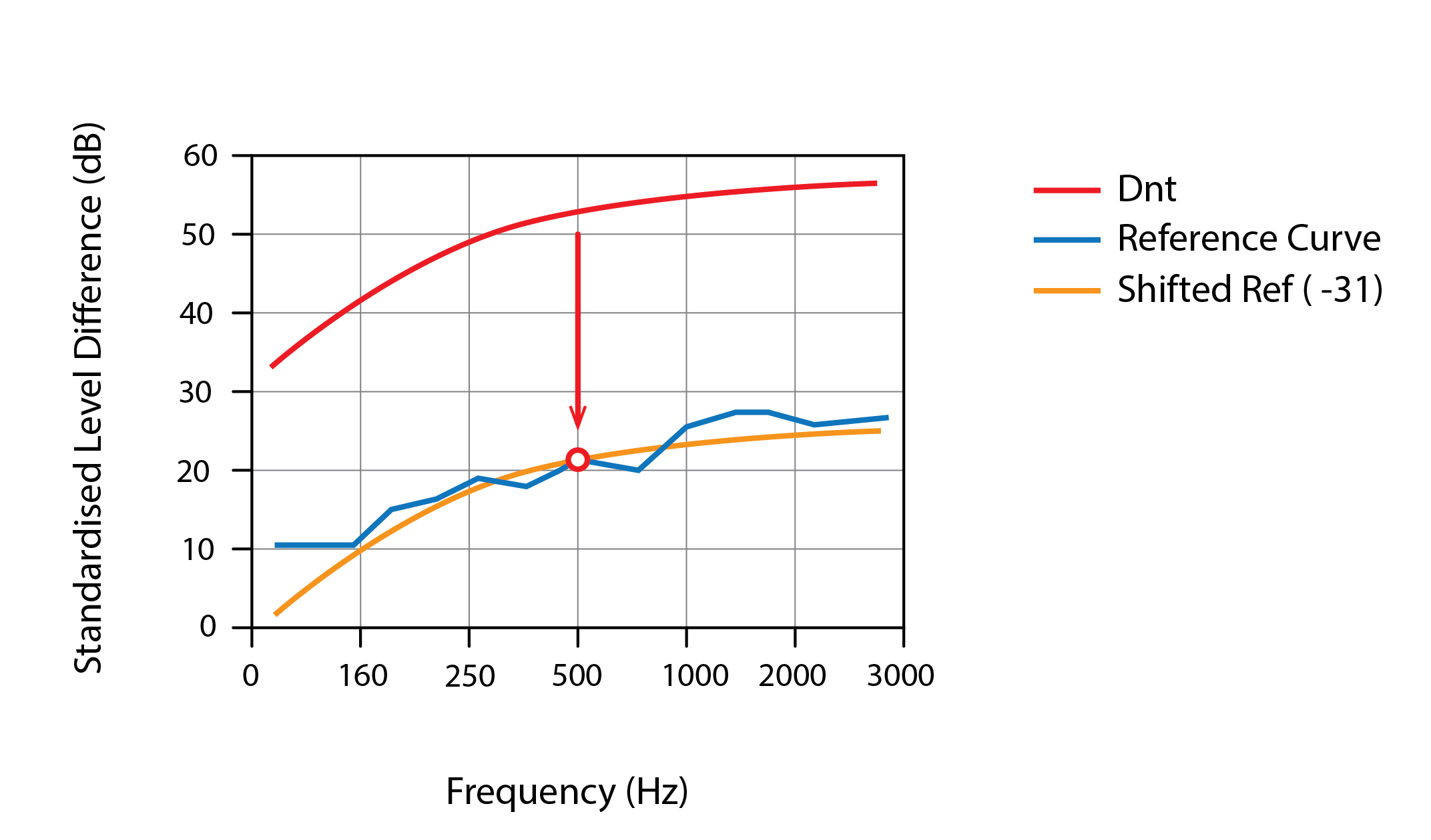
(9) $\begin{equation*} \left D_{nT} = L_s-L_r + 10 \log_{10} \frac {T}{T_o} \end{equation*}$

Values for D_nT are calculated for all one-third octave bands, in Hz (e.g. 63, 80, 100, 125, 160, 200, 250… – where numbers in bold refer to the octave bands and the others, the one-third octave bands) and plotted on a chart, with frequency on x and D_nT on y. This is represented by the thick blue curve in the chart below. This curve is then compared with a reference curve, indicated by the thick red curve below. This reference curve is then adjusted (in this case, lowered) in 1dB increments until the mean of the differences between the values of the two curves for all 1/3 octave bands is within 2dB. The weighted (w) final value for D_nT,w corresponds to the value of the adjusted reference curve at a frequency of 500Hz.

Figure 12: The weighting of the standardised level difference

This exercise of determining the metric D_nT,w for a construction assembly is normally carried out by acousticians with specialised test chambers, using speakers positioned within the source room, microphones positioned within the receiving room, and a sample of the partition installed at the junction between these two rooms (e.g. a floor or wall). Designers can then refer to these pre-measured values to determine whether their selected assembly meets the relevant standard’s requirements. Occasionally, where flanking pathways are expected to differ significantly from those in the testing environment, on-site measurements may be needed. These are conducted in a similar manner. In both cases, corrections are sometimes required to account for the size of the assembly at the interface and for any variations in the spectra of emitted sound.

8.4 Questions and worked examples

This section contains a series of worked examples or problems (P) and their solutions (S), as well as a series of written questions (Q) and their written answers (A).

P1) In an office room, you measure three different sounds, one at a time: talking (45dB), traffic noise from outside (35dB) and a quiet photocopier (25dB). What will be the total sound pressure level L when these are added together?

P2) If the photocopier is now switched off, but the traffic noise level increases to 45dB, what will be the new combined total value of L?

P3) An empty unfurnished office room has dimensions 6m wide, 5m deep and 3m high. The floors are carpeted ( $\alpha = 0.3$ @ 2kHz), the walls and ceiling are of painted plaster ( $\alpha = 0.02$ ) and there is a large 3m x 1.5m window ( $\alpha = 0.03$ ) in one wall. Calculate the reverberation time at 2kHz.

P4) Consider now a space of Church-like dimensions and surface finishes. The space measures 50m long, 25m wide and 15m high. All of the surfaces are stone ( $\alpha = 0.05$ ) and 10% of the walls are glazed ( $\alpha = 0.03$ ). Calculate the reverberation time, again at 2kHz.

S1) Our intensity ratios (the individual elements of equation 3 above) are 316, 3,162 and 31,623 for the 25dB, 35dB and 45dB sources respectively. Adding these together and converting back to the combined L_Tot we have 45.45dB.

S2) Combining the equal intensity ratios of 31,623 and converting back to L_Tot yields the expected total of 45+3dB, to give 48dB.

S3) The component parts of the room absorption (the right-hand side of equation 6) are as follows:

Surface type	Area, m²	Absorption coefficient (-)	Absorption
Glass	4.5	0.03	0.135
Wall	61.5	0.02	1.230
Floor	30.0	0.30	9.000
Ceiling	30.0	0.02	0.600
Total	126.0		10.965

The reverberation time then is $0.161 \cdot 90 / 10.965$ = 1.32 s.

S4) The component parts of the room absorption (the right-hand side of equation 6) are as follows:

Surface type	Area, m²	Absorption coefficient (-)	Absorption
Glass	225	0.05	11.25
Wall	2,025	0.03	60.75
Floor	1,250	0.05	62.50
Ceiling	1,250	0.05	62.50
Total	4,750		197

The reverberation time then is $0.161 \cdot 18,750 / 197$ = 15.32 s.

Q1) Comment on the suitability of our two spaces (the office and the church-like spaces) for the intelligibility of speech and the appreciation of organ music.

A1) The reverberation time in the church-like space is very long, excessively so for the speech from a single orator to be intelligible. In this case, it would be preferable to locate small speakers along the length of the space, to broadcast the speech to people seated (or standing) along its length. This space would however be well suited to the hosting of organ music. Conversely, the smaller office-type space has a reverberation time that is close to ideal for speech intelligibility, but it is acoustically what we refer to as quite a dead space, so that music would be less well appreciated.

References

Her Majesty’s Stationery Office (2015), Building Regulations – Approved Document E, 2015.

Department for Education (2015). Building Bulletin 93: Acoustic design of schools: performance standards, 2015.

8 Architectural acoustics

8.1 Principles of waves, sound and noise

8.2 Reverberation and intelligibility

8.3 Sound transmission and insulation

8.4 Questions and worked examples

References

Further reading

Licence

Share This Book